Introduction to Physics Informed Neural Networks

Introduction

This project here was meant to give a headstart on how to implement Physics-Informed-Neural-Networks. Before we head in, there are some dependencies to be installed. I did this project using Jupyter Notebooks and I would recommend anyone reading this do the same. You can install Jupyter in your PC or workstation natively (using Anaconda ) or use it online in Jypyter labs. In my case, I am it using from Anaconda.

If you are done setting up, Use the code below to setup the Python / Jupyter environment using conda:

conda create -n workshop python=3
conda activate workshop
conda install jupyter numpy matplotlib
conda install pytorch torchvision torchaudio -c pytorch

Once done, you can start by importing the basic libraries,

import torch
import torch.nn as nn
import numpy as np
import matplotlib.pyplot as plt

Coding a PINN from scratch

We will be coding a PINN from scratch in PyTorch and using it for simulation and inversion tasks related to the damped harmonic oscillator. Here, we are interested in modelling the displacement \(u(t)\) of the oscillator as a function of time which can be described by the differential equation:

where \(m\) is the mass of the oscillator, \(\mu\) is the coefficient of friction and \(k\) is the spring constant.

We will focus on solving the problem in an under-damped state i.e. where the oscillation is slowly damped by friction. Mathematically, this occurs when:

Furthermore, we consider the following initial conditions of the system:

For this particular case, the exact solution is given by:

Workflow Overview

There are two scientific tasks related to the harmonic oscillator we will ise a PINN for:

• First, we will simulate the system using a PINN with the given initial condition.
• Second, we will invert for underlying parameters of the system using a PINN, given some noisy observation from the oscillatiors displacement.
• Finally, we will investigate how well the PINN scales to higher frequency oscillations and what can be done to improve the convergence.

Initial Setup

First we define some helper functions

def exact_solution(d, w0, t):
    "Defines the analytical solution to the under-damped harmonic oscillatior problem above."
    assert d < w0
    w = np.sqrt(w0**2-d**2)
    phi = np.arctan(-d/w)
    A = 1/(2*np.cos(phi))
    cos = torch.cos(phi+w*t)
    exp = torch.exp(-d*t)
    u = exp*2*A*cos
    return u

class FCN(nn.Module):
    "Defines a standard fully-connected network in PyTorch"

    def __init__(self, N_INPUT, N_OUTPUT, N_HIDDEN, N_LAYERS):
        super().__init__()
        activation = nn.Tanh
        self.fcs = nn.Sequential(*[
                nn.Linear(N_INPUT, N_HIDDEN),
                activation()])
        self.fch = nn.Sequential(*[
                        nn.Sequential(*[
                            nn.Linear(N_HIDDEN, N_HIDDEN),
                            activation()]) for _ in range(N_LAYERS-1)])
        self.fce = nn.Linear(N_HIDDEN, N_OUTPUT)

    def forward(self, x):
        x = self.fcs(x)
        x = self.fch(x)
        x = self.fce(x)
        return x

Task 1: Train the PINN to simulate the system

The first task is to use a PINN to simulate the system

Specifically, our inputs and outputs are:

• Inputs: underlying differential equation and the initial conditions of the system
• Outputs: estimate the solution, \(u(t)\)

Approach

The PINN is trained to directly approximate the solution to the differential equation, i.e.

where \(\theta\) are the free parameters of teh PINN.

Loss Function

To simulate the system, the PINN is trained with the following loss function:

For this task, we use \(\delta=2\), \(\omega_0=20\), and try to learn the solution over the domain \(t \in [0,1]\).

Notes

The first two terms in the loss function represent the boundary loss, and tries to ensure that the solution learned by the PINN matches the initial conditions of the system, namely, \(u(t=0)=1\) and \(u^\prime(t=0)=0\).

The second term in the loss function is called the physics loss, and tries to ensure that the PINN solution obeys the underlying differential equation at a set of training points \([t_i]\) sampled over the entire domain.

The hyperparameters, \(\lambda_1\) and \(\lambda_2\), are used to balance the terms in the loss function, to ensure stability during training.

Auto-differentiation (torch.autograd) is ued to calculate the gradients of the PINN with respect to the input required to evaluate the loss function. This is vey powerful!

torch.manual_seed(123)

# define a neural network to train
# TODO: write code here
pinn = FCN(1,1,32,3)

# define boundary points, for the boundary loss
# TODO: write code here
t_boundary = torch.tensor(0.).view(-1,1).requires_grad_(True)

# define training points over the entire domainn, for the physics loss
# TODO: write code here
t_physics = torch.linspace(0,1,30).view(-1,1).requires_grad_(True)

# train the PINN
d, w0 = 2, 20
mu, k = 2*d, w0**2
t_test = torch.linspace(0,1,300).view(-1,1)
u_exact = exact_solution(d, w0, t_test)
optimiser = torch.optim.Adam(pinn.parameters(), lr=1e-3)
for i in range(15001):
    optimiser.zero_grad()

    # compute each term of the PINN loss function above
    # using the following hyperparameters
    lambda1, lambda2 = 1e-1, 1e-4

    # compute boundary loss
    # TODO: write code here
    u = pinn(t_boundary) # (1,1)
    loss1 = (torch.squeeze(u) - 1)**2

    dudt = torch.autograd.grad(u, t_boundary, torch.ones_like(u), create_graph=True)[0]
    loss2 = (torch.squeeze(dudt) - 0)**2

    # compute physics loss
    # TODO: write code here
    u = pinn(t_physics)
    dudt = torch.autograd.grad(u, t_physics, torch.ones_like(u), create_graph=True)[0]
    d2udt2 = torch.autograd.grad(dudt, t_physics, torch.ones_like(dudt), create_graph=True)[0]
    loss3 = torch.mean((d2udt2 + mu*dudt + k*u)**2)


    # backpropagate joint loss, take optimiser step
    # TODO: write code here
    loss = loss1 + lambda1*loss2 + lambda2*loss3
    loss.backward()
    optimiser.step()

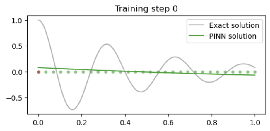
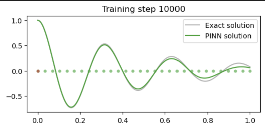
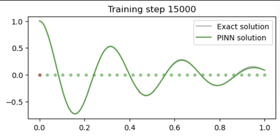
    # plot the result as training progresses
    if i % 5000 == 0:
        #print (u.abs().mean().item(), dudt.abs().item(), d2udt2.abs().mean().item())
        u = pinn(t_test).detach()
        plt.figure(figsize=(6,2.5))
        plt.scatter(t_physics.detach()[:,0],
                    torch.zeros_like(t_physics)[:,0], s=20, lw=0, color="tab:green", alpha=0.6)
        plt.scatter(t_boundary.detach()[:,0],
                    torch.zeros_like(t_boundary)[:,0], s=20, lw=0, color="tab:red", alpha=0.6)
        plt.plot(t_test[:,0], u_exact[:,0], label="Exact solution", color="tab:grey", alpha=0.6)
        plt.plot(t_test[:,0], u[:,0], label="PINN solution", color="tab:green")
        plt.title(f"Training step {i}")
        plt.legend()
        plt.show()

Task 2: Train a PINN to invert for underlying parameters

Task

The second task is to use a PINN to invert for underlying parameters.’

Specifically, our inputs and outputs are:

• Inputs: noisy observations of the oscillator’s displacement
• Outputs: estimate \(\mu\), the coefficient of friction

Approach

Similar to above, the PINN is trained to directly approximate the solution to the differential equation, i.e. \(u_{PINN}(t; \theta) \approx u(t),\) where $\theta$ are the free parameters of the PINN.

The key idea here is to also treat $\mu$ as a learning parameter when training the PINN - so that we both simulate the solution and invert for this parameter.

Loss Function

The PINN is trained with a slightly different loss function: \(\mathcal{L}(\theta, \mu) = \frac{1}{N} \sum^N_i \bigg ( \bigg [ m \frac{d^2}{dt^2} + \mu \frac{d}{dt} + k \bigg ] u_{PINN}(t_i; \theta) \bigg )^2 + \frac{\lambda}{M} \sum^M_j (u_{PINN}(t_j; \theta) - u_{obs}(t_j))^2\)

Notes

There are two terms in the loss function here. The first is the physics loss, formed in the same way as above, which hensures the solution learned by the PINN is consistent with the known physics.

The second term is called the data loss, and makes sure that the solution learned by the PINN fits the (potentially noisy) observations of the solution that are available.

Note, we have removed the boundary loss term, as we do not know these (i.e. we are only given the observed measurements of the system).

In this setup, the PINN parameters \(\theta\) and \(\mu\) are jointly learned during the optimization.

Again, auto-differentiation is our friend and will allow us to easily define this problem!

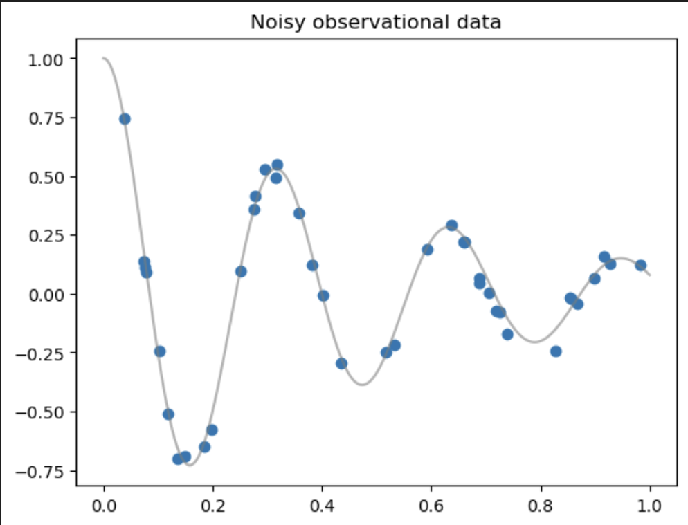
# first, create some noisy observational data
torch.manual_seed(123)
d, w0 = 2, 20
print(f"True value of mu: {2*d}")
t_obs = torch.rand(40).view(-1,1)
u_obs = exact_solution(d, w0, t_obs) + 0.04*torch.randn_like(t_obs)

plt.figure()
plt.title("Noisy observational data")
plt.scatter(t_obs[:,0], u_obs[:,0])
t_test, u_exact = torch.linspace(0,1,300).view(-1,1), exact_solution(d, w0, t_test)
plt.plot(t_test[:,0], u_exact[:,0], label="Exact solution", color="tab:grey", alpha=0.6)
plt.show()

Output

True value of mu: 4

torch.manual_seed(123)

# Define a neural network to train
pinn = FCN(1,1,32,3)

# define training points over the entire domain, for the physics loss
t_physics = torch.linspace(0,1,30).view(-1,1).requires_grad_(True)

# train the PINN
d, w0 = 2, 20
_ , k = 2*d, w0**2

# create mu as a learnable parameter
# TODO: write code here

mu = torch.nn.Parameter(torch.zeros(1, requires_grad=True))
mus = []

# add mu to the optimiser
# TODO: write code here

optimiser = torch.optim.Adam(list(pinn.parameters())+[mu],lr=1e-3)

for i in range(15001):
    optimiser.zero_grad()

    # compute each term of the PINN loss function above
    # using the following hyperparameters:
    lambda1 = 1e4

    # compute physics loss
    u = pinn(t_physics)
    dudt = torch.autograd.grad(u, t_physics, torch.ones_like(u), create_graph=True)[0]
    d2udt2 = torch.autograd.grad(dudt, t_physics, torch.ones_like(dudt), create_graph=True)[0]
    loss1 = torch.mean((d2udt2 + mu*dudt + k*u)**2)

    # compute data loss
    # TODO: write code here
    u = pinn(t_obs)
    loss2 = torch.mean((u-u_obs)**2)

    # backpropagate joint loss, take optimiser step
    loss = loss1 + lambda1*loss2
    loss.backward()
    optimiser.step()

    # record mu value
    # TODO: write code here
    mus.append(mu.item())

    # plot the result as training progresses
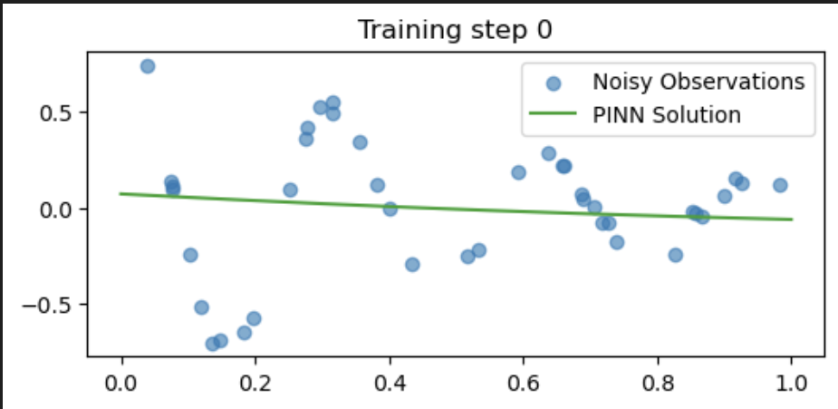
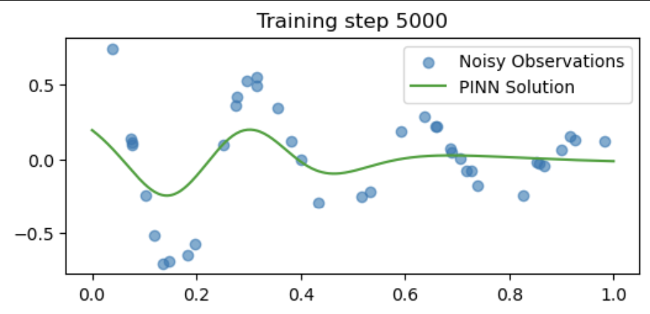
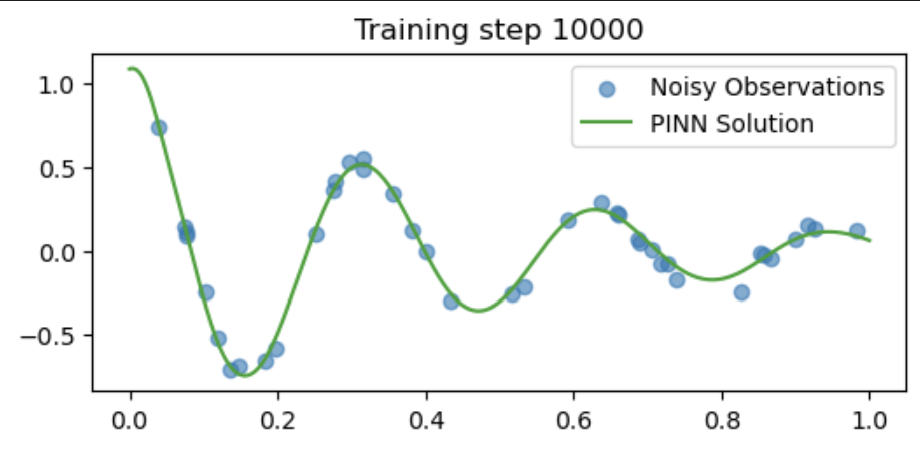
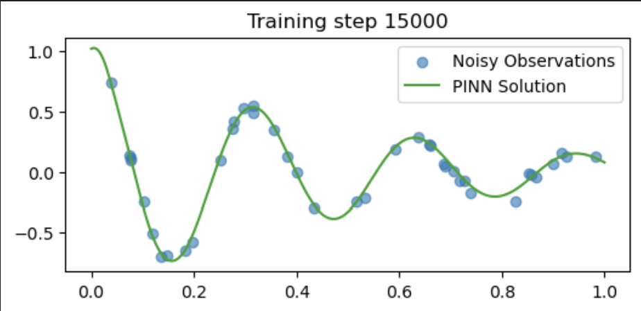
    if i % 5000 == 0:
        u = pinn(t_test).detach()
        plt.figure(figsize=(6,2.5))
        plt.scatter(t_obs[:,0], u_obs[:,0], label="Noisy Observations", alpha=0.6)
        plt.plot(t_test[:,0], u[:,0], label="PINN Solution", color="tab:green")
        plt.title(f"Training step {i}")
        plt.legend()
        plt.show()

plt.figure()
plt.title("$\mu$")
plt.plot(mus, label="PINN estimate")
plt.hlines(2*d, 0, len(mus), label="True value", color="tab:green")
plt.legend()
plt.xlabel("Training step")
plt.show()