Introduction

OpenFOAM (Open Field Operation and Manipulation) is a popular open-source CFD toolbox known for its flexibility and extensibility. Unlike commercial software, OpenFOAM allows users to modify the source code and implement custom functionality, making it highly suitable for academic research and specialized industrial applications. Among its many capabilities, OpenFOAM supports the development of custom function objects, which enable users to perform advanced calculations or derive new fields during simulations.

This project involves creating a new solver named scalarFoam based on the Navier-Stokes and the SIMPLE algorithm to incorporate the temperature equation setting up a case file for the shock tube problem with appropriate initial and boundary conditions, and simulating the heat transport alongside the fluid flow i.e. Convection and Diffusion phenomenon with various conditions. The results are analyzed to confirm the solver’s performance using various schemes with the specified conditions.

Methodology

Solver Literature

The current solver implementation is similar and referenced from the previous work, where we have implemented a custom solver to incorporate the scalar quantity of Temperature. The scalarFoam solver we are going to implement is based on the general scalar transport equation where the scalar quantity here is Temperature T given below:

where,

• u is the velocity,
• T is the Temperature and
• DT is the Diffusion coefficient

Solver Implementation

A convection-diffusion scalar transport equation without source terms is implemented and solved by the scalarFoam solver.

The solver’s primary characteristics are:

• Solving a convection-diffusion equation using boundary conditions that the user specifies
• User-provided arbitrary velocity and scalar field that is read at runtime

The finite volume technique serves as the foundation for the numerical approach utilized to solve the scalar transport problem in scalarFoam. Specifically, the fvm family of operators is used to implicitly discretize all the equations’ terms.

Because of its sophisticated C++ syntax and its structure, OpenFOAM makes it simple to implement a scalar transport equation. To specify the fields involved in the terms of the transport equation, however, a few preparatory procedures are required. Generally in OpenFOAM, the solver directory contains the main driver program, in our case, scalarFoam.C, required fields (flow variables) to be read in createFields.H and Make files which help in compiling the solver with the necessary dependencies.

Make files

In the Make files, files show the location of the solver and options contain the full directory paths to locate the header files to compile the solver shown below:

Make/files:

 scalarFoam.C
 EXE = $(FOAM
 USER
 APPBIN)/scalarFoam

Make/options:

 EXE INC = \
 -I$(LIB SRC)/finiteVolume/lnInclude \
 -I$(LIB SRC)/meshTools/lnInclude \
 -I$(LIB SRC)/sampling/lnInclude
 
 EXE LIBS = \
 -lfiniteVolume \
 -lfvOptions \
 -lmeshTools \
 -lsampling

For our solver, we need finite volume numerics, meshing and sampling libraries and therefore require the necessary header files, specified by the EXE_INC = -I option, and links to the libraries with theEXE_LIBS = -l option.

createFields.H

Now, we move onto the createFields.H, which contains the necessary variables in the Eq. to be read by OpenFOAM for our solver. The variables we need are Velocity U, Temperature T and the diffusion coefficient DT which are shown in the code below:

Temperature:

Info << ”Reading field T\n” << endl;\\
 volScalarField T
 (
	 IOobject
	 (
		 "T",
		 runTime.timeName(),
		 mesh,
		 IOobject ::MUSTREAD,
		 IOobject ::AUTOWRITE
	 ),
	 mesh
 );

Velocity:

 Info<< ”Reading field U\n” << endl;
 volVectorField U
 (
	 IOobject
	 (
		 "U",
		 runTime.timeName(),
		 mesh,
		 IOobject ::MUSTREAD,
		 IOobject ::AUTOWRITE
	 ),
	 mesh
 );

Diffusion Coefficient:

 Info<< ”Reading transportProperties\n” << endl ;
 IOdictionary transportProperties
 (
	 IOobject
	 (
		 "transportProperties",
		 runTime.constant (),
		 mesh,
		 IOobject ::MUST READ IF MODIFIED,
		 IOobject ::NOWRITE
	 )
 );
 Info<< ”Reading diffusivity DT\n” << endl;
 dimensionedScalar DT("DT", dimViscosity, transportProperties );

As part of the OpenFOAM writing structure, we add the info statements so that when we run the solver, we know that the variables are being read out to the user. The structure rules also dictates to include necessary header files for the files to be read into and integrate with the finite volume methodology.

scalarFoam.C

We now move onto creating our main solver code.

Info<< ”\nCalculating scalar transport\n” << endl ;
	#include ”CourantNo.H”
	while (simple . loop ())
	{
		Info<< ”Time=” << runTime.timeName() << nl << endl;
		while (simple . correctNonOrthogonal ())
		{
			fvScalarMatrix TEqn
			(
		          fvm :: ddt(T)
				+ fvm:: div(phi , T)
				− fvm:: laplacian (DT, T)
				==
				fvOptions(T)
			);
			TEqn. relax ();
			fvOptions . constrain (TEqn);
			TEqn. solve ();
			fvOptions . correct (T);
		}
		runTime. write ();
	}
 Info<< ”End\n” << endl ;

where the matrix resulting from the discretization of the scalar transport equation is contained in a fvScalarMatrix object and solved using the solution() function. Because it makes it simple to add terms to the transport equations based on user requirements, this syntax is more general.

The solver setup is complete, now using the wmake command, we compile the solver and integrate it into the OpenFOAM user defined solvers.

Numerical Schemes

Diffusion Schemes

Diffusion represents the process by which temperature spreads due to molecular interactions, independent of fluid motion. It is governed by the diffusion coefficient DT.

Diffusion Setup in the Study:

• Velocity is set to zero (U = 0,0,0) in the setFieldsDict.
• The diffusion coefficient DT is varied with values:
  • 0 (no diffusion)
  • 0.0001 (low diffusion)
  • 0.01 (moderate diffusion)
  • 1 (high diffusion)

By simulating these cases, we compare contour plots of temperature distribution to understand the effect of diffusion.

Convection Schemes

Convection is the transport of temperature due to fluid motion. Different numerical schemes handle the convection term in the governing equations differently, affecting accuracy and numerical stability.

Schemes Used in the Study:

• Upwind: A first-order scheme that ensures stability but introduces numerical diffusion, which smears sharp gradients.
• LinearUpwind: A second-order accurate scheme that reduces numerical diffusion compared to the upwind method.
• Quadratic: Uses higher-order interpolation to improve accuracy while maintaining stability.
• Cubic: Further refines the interpolation, capturing sharper gradients with minimal diffusion.
• vanLeer: A flux-limiter scheme that adapts between first and second order for better accuracy and stability.
• QUICK (Quadratic Upstream Interpolation for Convective Kinematics)– A third order accurate scheme that provides better accuracy while reducing numerical oscillations.

Each of these schemes will be tested by setting x-velocity (U = 1,0,0) in the setFieldsDict with no diffusion and observing the transport of an initial temperature block along the length of the tube.

This study helps understand the balance between numerical diffusion and accuracy, ensuring appropriate scheme selection for convection-diffusion problems in computational fluid dynamics (CFD) simulations.

Simulation and Solution Setup

As proposed, we will be using the 1D-shocktube case for doing the case study. For that, we first copy the tutorial case to our current folder with the following command:

cp-r $FOAM_TUTORIALS/compressible/sonicFoam/laminar/shockTube $FOAM_RUN

And we will use the controlDict, fvSchemes and fvSolution from $FOAM_TUTORIALS/basic/scalarTransportFoam/pitzDaily case.

The file structure for the shocktube case is given below:

 |−− 0
	 |−− T
	 |−− U
 |−− constant
	 |−− polyMesh
	 |−− blockMeshDict
	 |−− transportProperties
 |−− system
	 |−− controlDict
	 |−− fvSchemes
	 |−− fvSolution
	 |−− setFieldsDict

We will initialize the center of the tube with a block of temperature equal to a certain value and then see how this temperature convects, when different convection schemes are applied:

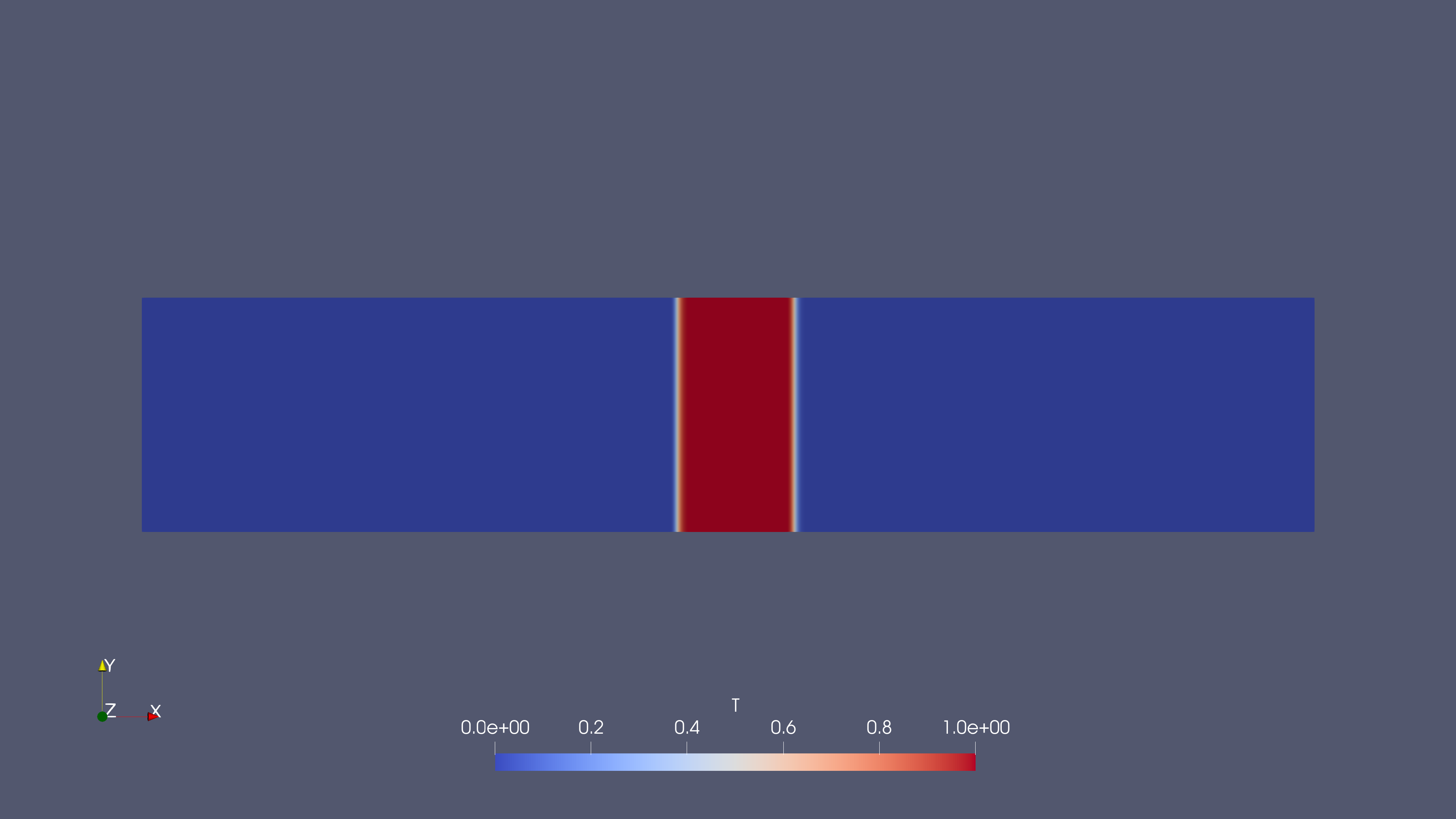                  Figure 1: Initial Condition for Temperature

We will use the setFields utility to initialize this block of temperature in the center with T as 1.0 Kelvin.

FoamFile
 {
	version		2.0;
	format		ascii;
	class		disctionary;
	object 		setFieldsDict;
 }
 // ∗ ∗ ∗ ∗ ∗ ∗ ∗ ∗ ∗ ∗ ∗ ∗ ∗ ∗ ∗ ∗ ∗ ∗ ∗ ∗ ∗ ∗ ∗ ∗ ∗ ∗ ∗ ∗ ∗ ∗ //
 
defaultFieldValues
 (
	 volVectorFieldValue U (0 0 0)
	 volScalarFieldValue T 0
 ) ;
regions
(
	boxToCell
	{
		box (−0.5 −1 −1) (0.5 1 1);
		fieldValues
		(
			volScalarFieldValue T 1.0
		);
	}
);

These cases are simulated for t = 5 seconds with the same blockMesh settings as in the original sonicFoam tutorial. Refer to the controlDict file in the Appendix section.

Initial & Boundary Conditions

We have only three variables to consider, Temperature, Velocity and the Diffusion coefficient for which we set the conditions shown below:

Temperature `0/T`:

dimensions      [0 0 0 1 0 0 0];

internalField   uniform 1;

boundaryField
{
    sides
    {
        type            zeroGradient;
    }
    empty
    {
        type            empty;
    }
}

Velocity `0/U`:

dimensions      [0 1 -1 0 0 0 0];

internalField   uniform (0 0 0);

boundaryField
{
    sides
    {
        type            zeroGradient;
    }
    empty
    {
        type            empty;
    }
}

For pure diffusion case, the velocity is going to be 0 while for pure convection, we set the velocity through setFieldsDict which automatically updates the 0/U file with the given velocity value of 1 m/s.

constant/transportProperties: And, we set the diffusion coefficient DT through the transportProperties file below

DT		 DT [0 2 −1 0 0 0 0] 0;

The value highlighted in red in the above code is where the diffusion coefficient is given. For the pure diffusion cases, we set the given coefficient values and run the cases for comparison. For the pure convection cases, we naturally set the value to 0.

Solution Control

For the pure diffusion cases, we don’t need to change anything in solution control.But, for pure convection cases, we need to change the discretization schemes for the temperature divergence term in fvSchemesas shown below:

divSchemes
 {
	default			none;
	div (phi ,T)	Gauss linearUpwind grad(T);
 }

The above example showcases the implementation of linearUpwind scheme. Similarly, we change the schemes as needed for the comparison of the convective behavior.

Beyond this, all the settings the cases remain the same. Once the setup is done, we finally run the simulation with the commands:

• blockMesh: Creates the geometry and the mesh
• checkMesh: Checks if the mesh has been properly implemented
• setFields: Sets the block of temperature in the tube
• scalarFoam: Runs the Solver

Results & Observations

Once the simulation is done, we post-process the results in Paraview.

Diffusion Cases

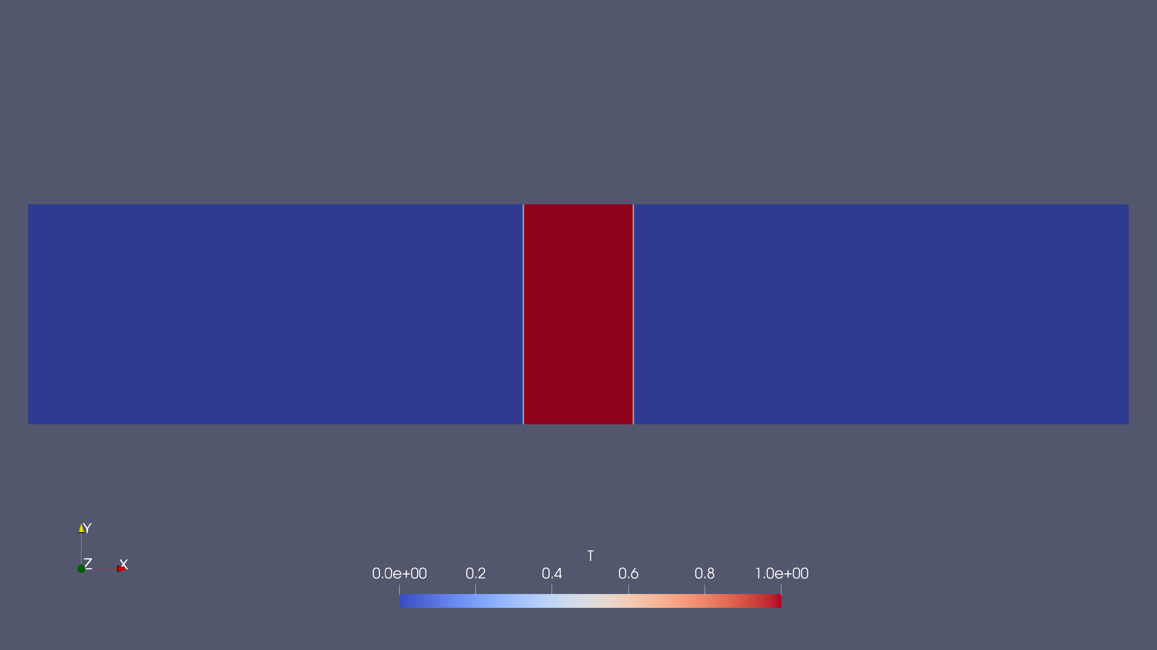                  Figure 2(a): Initial Shocktube Contour

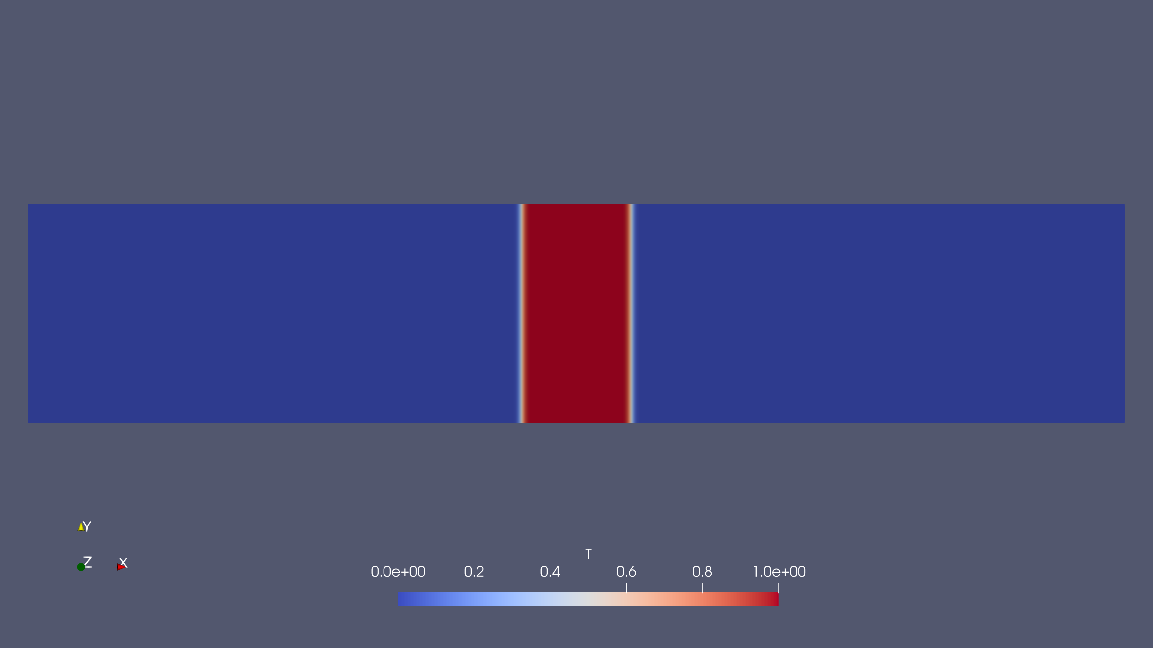                        Figure 2(b): DT=0.0001

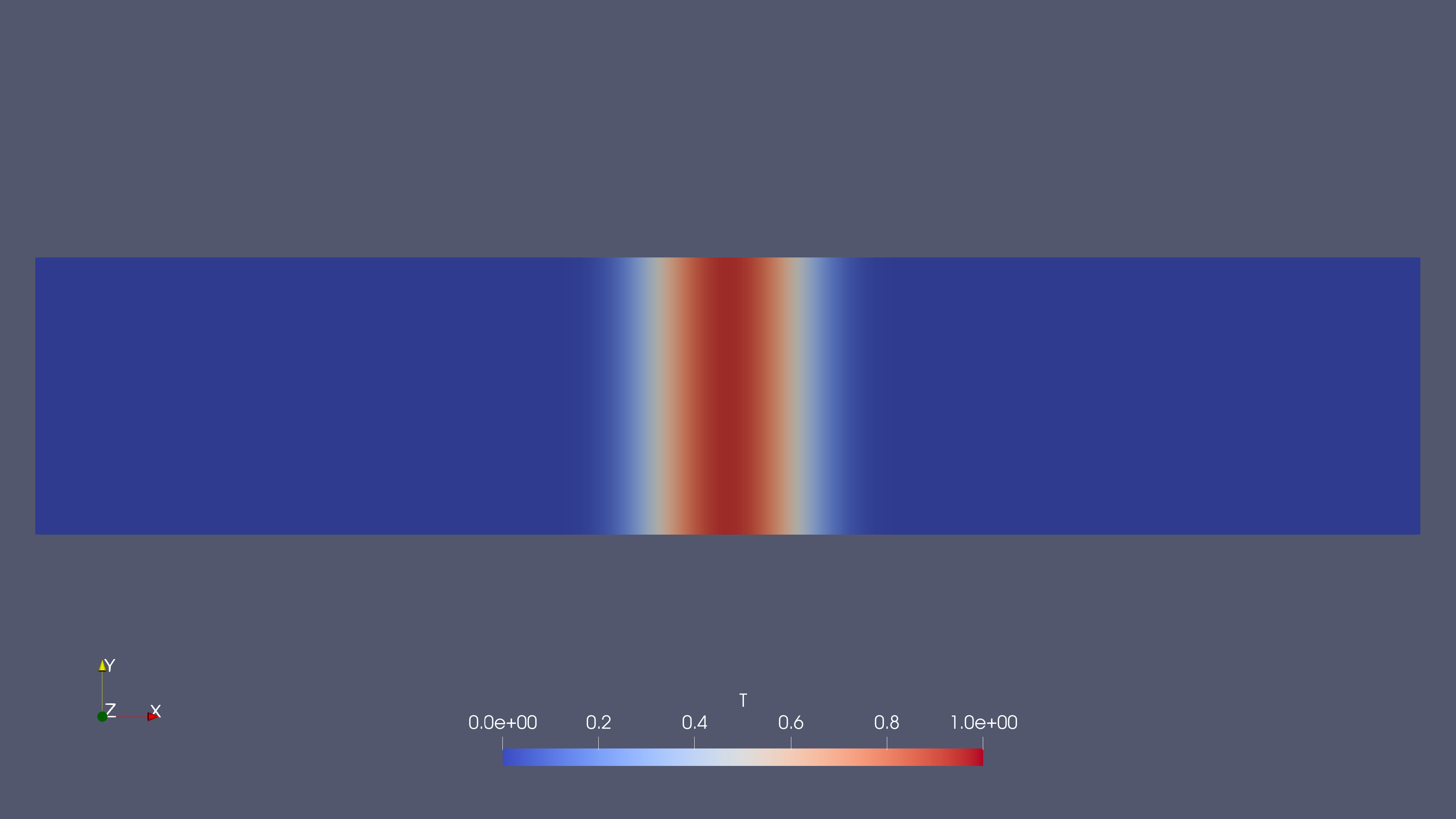                        Figure 2(c): DT=0.01

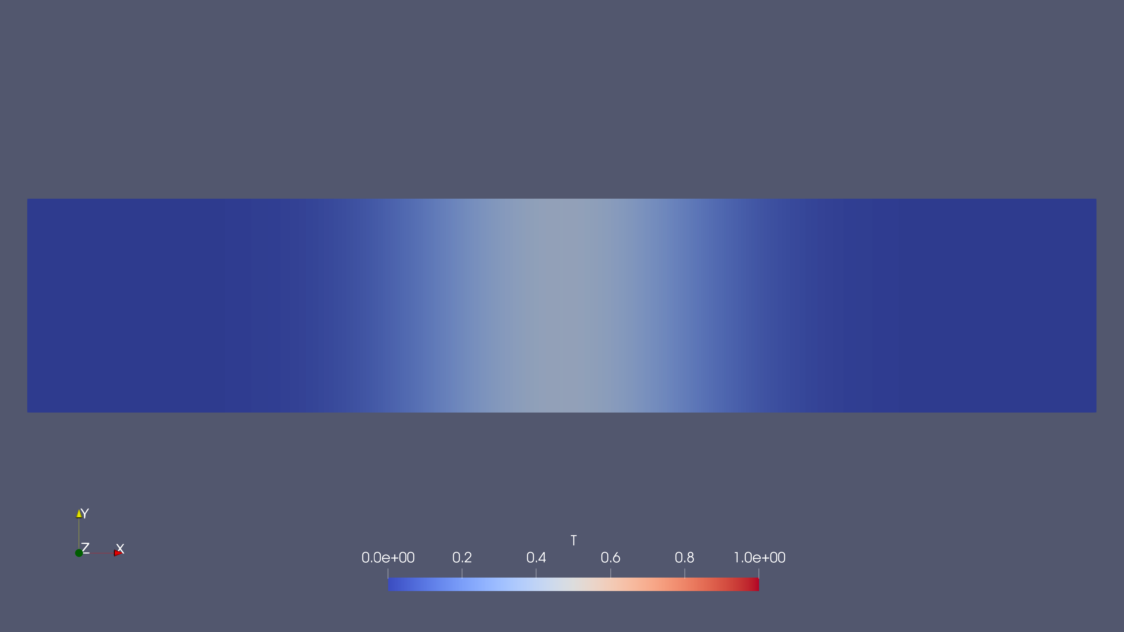                        Figure 2(d): DT=1

The simulations executed show the temperature diffusion behavior for different values of the diffusion coefficient DT (0, 0.0001, 0.01, and 1). Below are the key observations from the results:

• DT =0 (No Diffusion)
  • The initial condition remains unchanged throughout the simulation.
  • The temperature block retains its sharp boundaries, indicating that without diffusion, temperature does not spread beyond the initialized region.
  • This case represents an undisturbed temperature field (velocity is zero).
• DT =0.0001 (Minimal Diffusion)
  • Very slight spreading of the temperature profile is observed, but the central high-temperature region is still well-preserved.
  • The diffusion effect is nearly negligible, showing only minimal temperature gradient smoothing at the edges.
  • This suggests that in cases with very low diffusion, sharp temperature fronts can still persist.
• DT =0.01 (Moderate Diffusion)
  • The temperature gradient becomes smoother compared to lower DT values.
  • The temperature front begins to widen significantly, indicating more noticeable thermal diffusion.
  • While some of the initial sharpness is lost, the temperature field still retains a fairly distinct high-temperature region.
• DT =1 (High Diffusion)
  • Significant spreading of temperature is evident, with a broad and smooth transition from high to low temperatures.
  • The high-temperature region is no longer concentrated in the center but has diffused widely across the domain.
  • This case represents a diffusion-dominant scenario where conduction spreads heat uniformly over time.

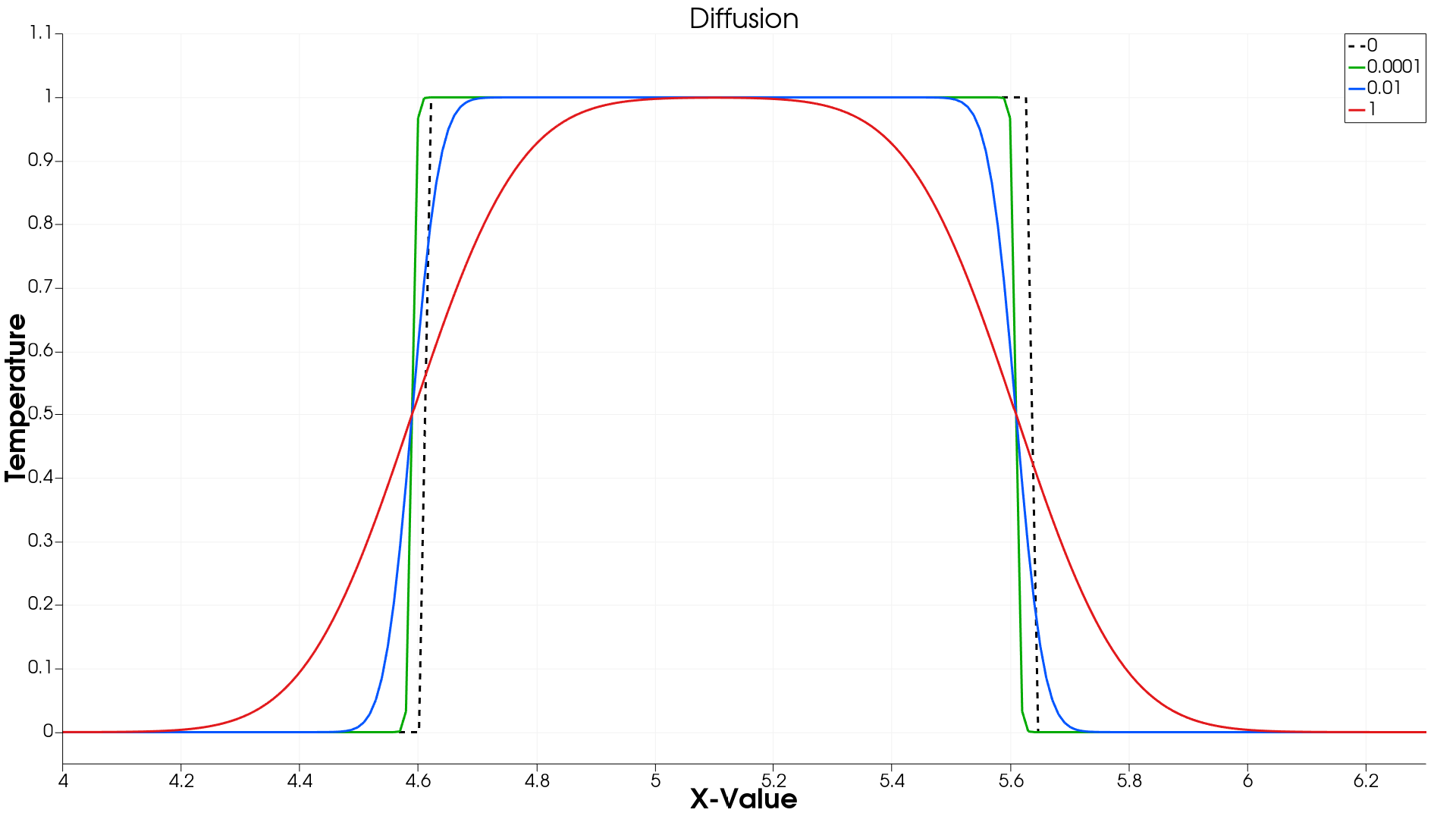                        Figure 3(a): DT at t = 0 sec

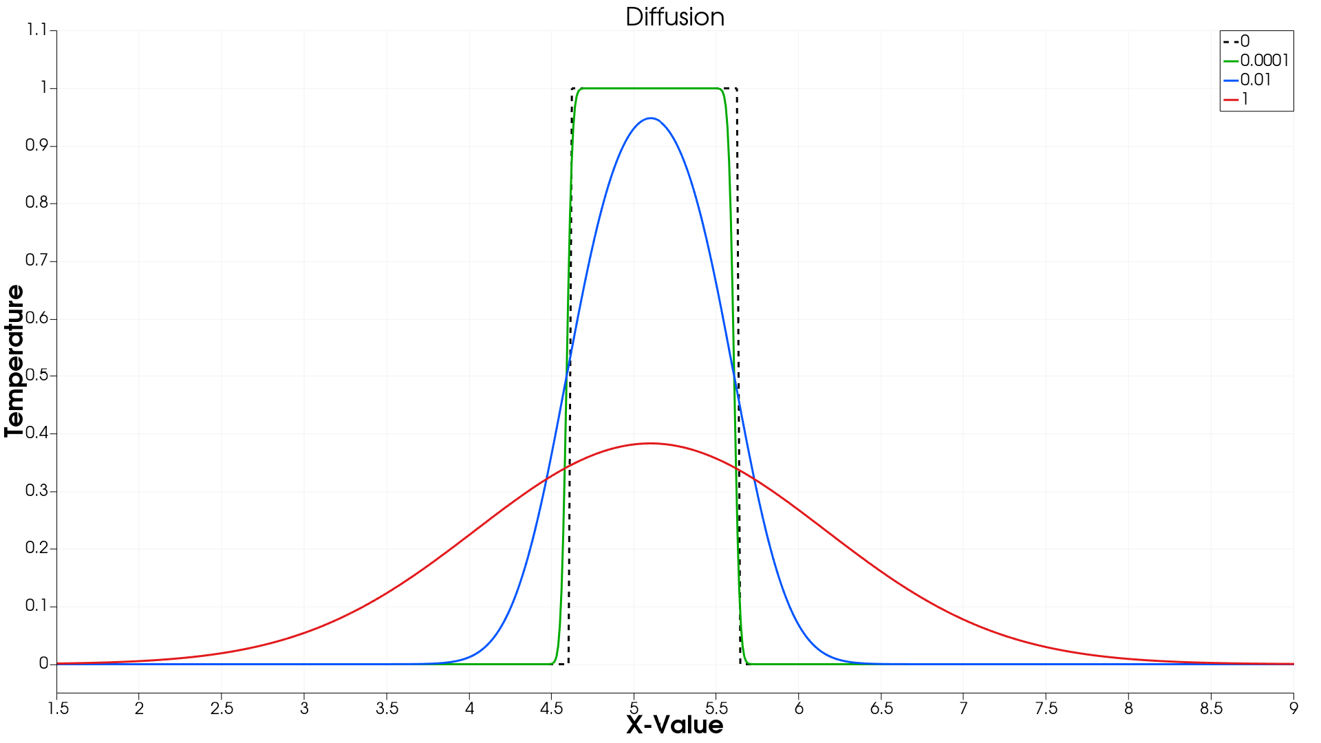                        Figure 3(a): DT at t = 5 sec

Observations from Temperature Profiles:

1. Initial Condition (t = 0 s):
   • The temperature profile starts as a sharp rectangular block, representing a well-defined temperature gradient.
   • Since diffusion has not yet occurred, all cases, regardless of DT, have identical profiles at t = 0.
2. Final Condition (t = 5 s):
   • As diffusion progresses, the temperature block spreads out depending on the magnitude of DT.
   • The temperature profile comparison graph at t = 5 s shows the effect of increasing DT on temperature spread.
3. Detailed Effects of Varying DT:
   • DT = 0 (No Diffusion)
     • The temperature block remains unchanged, retaining sharp edges.
   • DT = 0.0001 (Minimal Diffusion)– Aslight smoothing effect is observed at the temperature edges.
     • The profile remains close to the initial sharp block but with minimal rounding at the corners.
   • DT = 0.01 (Moderate Diffusion)
     • Anoticeable smoothing occurs, with the sharp edges gradually fading.
     • The temperature field expands further, reducing the central peak but maintaining a distinct region of high temperature.
   • DT = 1 (High Diffusion)
     • The temperature profile is significantly spread out, resembling a Gaussian distribution.
     • The high-temperature region is no longer concentrated, indicating a dominant diffusion effect leading to uniform temperature distribution.

Convection Cases

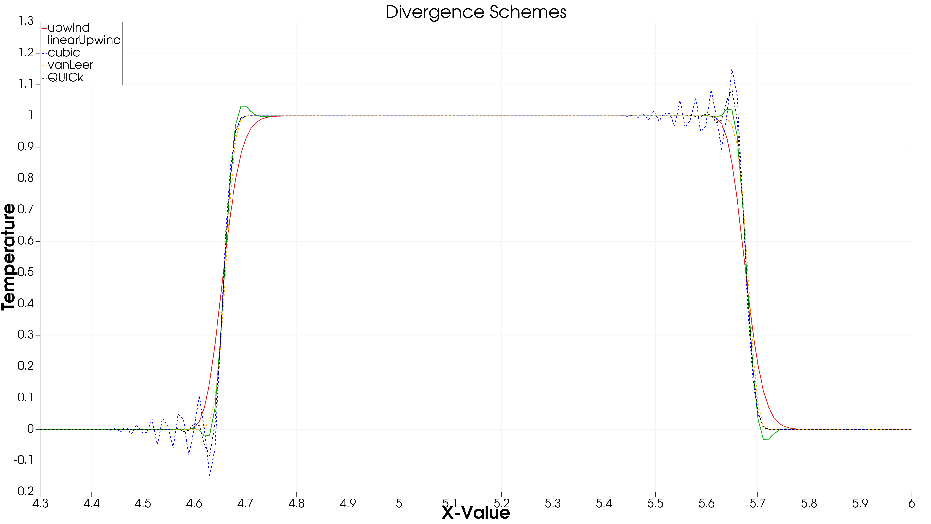                        Figure 3(a): Divergence Schemes at t = 0 sec

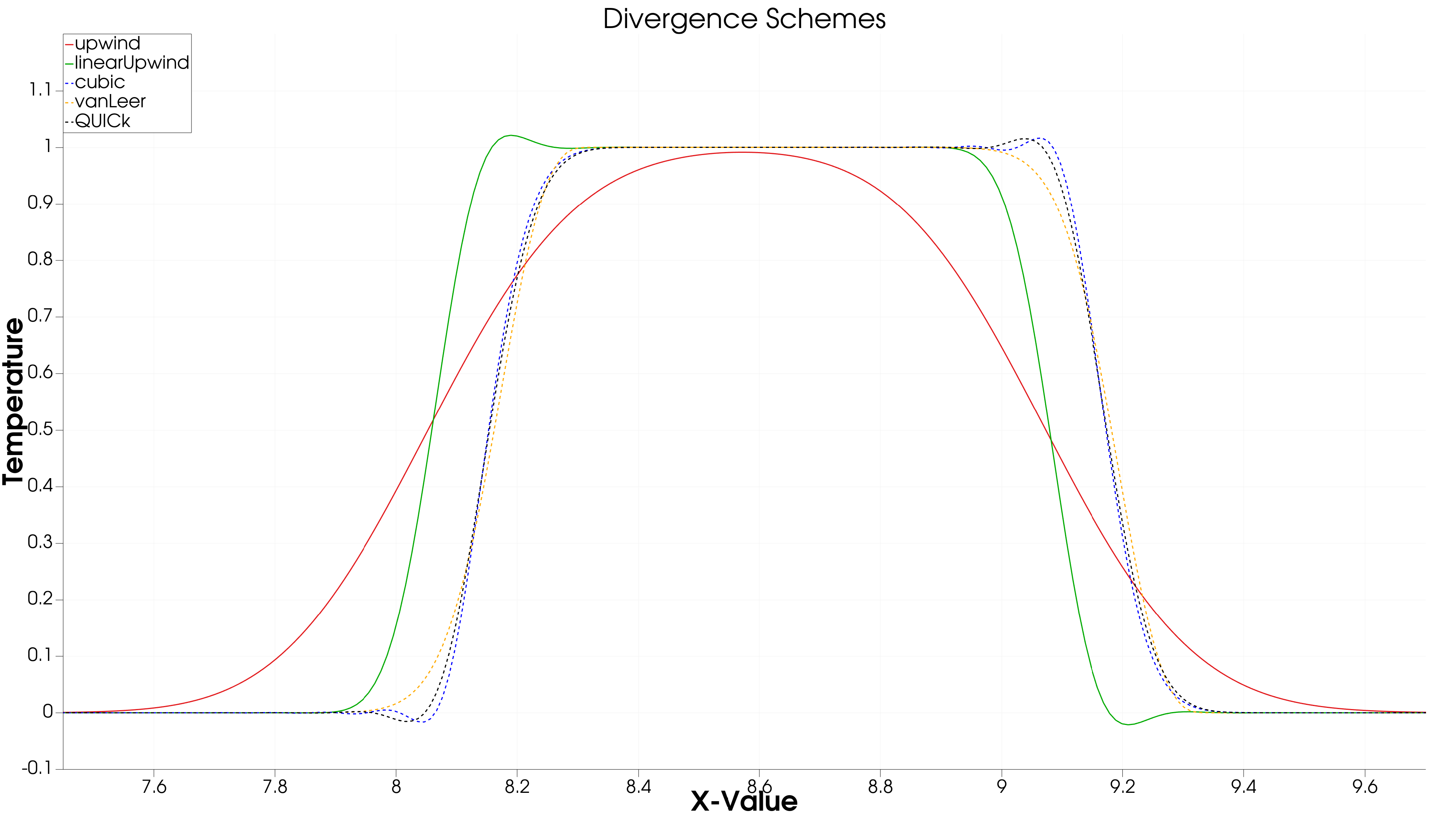                        Figure 3(a): Divergence Schemes at t = 5 sec

1. Initial Condition (t = 0 s):
   • The temperature distribution starts as a sharp block, with well-defined edges.
   • All schemes begin with the same profile since no numerical diffusion or dispersion has occurred yet.
2. Final Condition (t = 5 s)
   • Different discretization schemes affect how the temperature profile evolves over time.
   • The temperature profile comparison graph at t = 5s highlights the impact of different divergence schemes.
3. Detailed Effects of Different Divergence Schemes:
   • Upwind Scheme (First-Order)
     • Produces a smooth profile with noticeable numerical diffusion.
     • Sharp edges are smeared, leading to significant loss of temperature gradients.
     • Ensures stability but at the cost of lower accuracy.
   • Linear Upwind (Second-Order)
     • Retains sharper temperature fronts compared to the upwind scheme.
     • Some minor oscillations appear, indicating better accuracy but less damping of numerical errors.
   • Cubic Interpolation
     • Provides a sharper temperature front but introduces oscillations near discontinuities.
     • The oscillations (numerical ringing) suggest possible instability in high gradient regions.
   • VanLeer Scheme
     • A flux limiter scheme that balances between accuracy and stability.
     • Shows sharper gradients than the upwind scheme, but avoids excessive oscillations.
   • QUICK (Third-Order Upstream Scheme)
     • Produces one of the most accurate temperature profiles with minimal numerical diffusion.
     • However, some oscillations appear, particularly near steep gradients.

Conclusion

Diffusion Cases

1. Higher DT leads to faster and wider temperature spread, with a transition from a sharp profile to a smooth, diffused state.
2. For low DT values, temperature gradients remain steep, making higher-resolution schemes necessary for accurate numerical modeling.
3. For high DT, diffusion dominates over convection, leading to a more uniform heat distribution across the domain.
4. The comparison graphs at t = 0 s and t = 5 s confirm the theoretical expectation that diffusion progressively smoothens the temperature gradient over time.

These results help in selecting appropriate DT values in computational models, depending on whether diffusion effects need to be emphasized or minimized in a simulation.

Convection Cases

1. The Upwind scheme is the most stable but introduces significant numerical diffusion, making it unsuitable for capturing sharp temperature gradients.
2. Higher-order schemes (Cubic, QUICK) provide better accuracy but may introduce oscillations that can lead to numerical instability.
3. The vanLeer scheme provides a good balance between accuracy and stability, making it a preferable choice in many convection-dominated problems.
4. For high-resolution simulations, linearUpwind or QUICK may be preferred, but careful handling of oscillations is required.

These results emphasize the trade-off between accuracy, numerical diffusion, and stability, guiding the choice of discretization schemes based on the problem’s requirements.

The entire solver code and the case data can be accessed here here. This simulation was performed in Ubuntu 24.04 LTS using the Windows Subsystem for Linux utility on a Windows 11 system.