
Approximation of 2D Boussinesq Systems Using PINN
Published:
Authors: Ruthwik Nadam\(^1\), Sai Ujjwal Kanth Nandula\(^2\)
1. Central Michigan University, 2. University at Buffalo (SUNY)
Abstract
This Study focuses on approximating the 2-D incompressible buoyancy driven fluid flows incorporating Boussinesq Navier Stokes equations along with the advection equation with the help of Physics informed Neural Networks (PINNS) and an open-source library DeepXDE. The module DeepXDE is specifically built for PINNs and can be used to solve ordinary differential equations, partial differential equations and integro-differential equations. DeepXDE also provides the framework for operator learning networks (DeepONet).The main aim of this project is to build a neural network model respecting the laws of physics and governing the boundary and initial conditions to solve the partial differential equations. The difference in the losses when used different sampling techniques is observed. The loss value when used Latin Hypercube sampling is more than 1000 times when compared to a uniformly equally spaced sampling points.
Introduction
Boussinesq Equations
Boussinesq Navier-Stokes equations are non-linear partial differential equations. An extension of Navier-Stokes equations which are used to study the dynamics of buoyancy-driven fluid flows. These equations also account for the buoyancy effects due to the temperature variations in the fluid where the general Navier-Stokes equation do not. The equations are used in several applications such as meteorology, oceanography, and engineering to model natural convection. Equations such as the Navier-Stokes and its extension do not have an exact solution because of its highly non-linear terms. Traditional numerical methods which include finite element methods and finite volume methods are generally used to solve them but requires high computational resources and complex coding of boundary conditions.
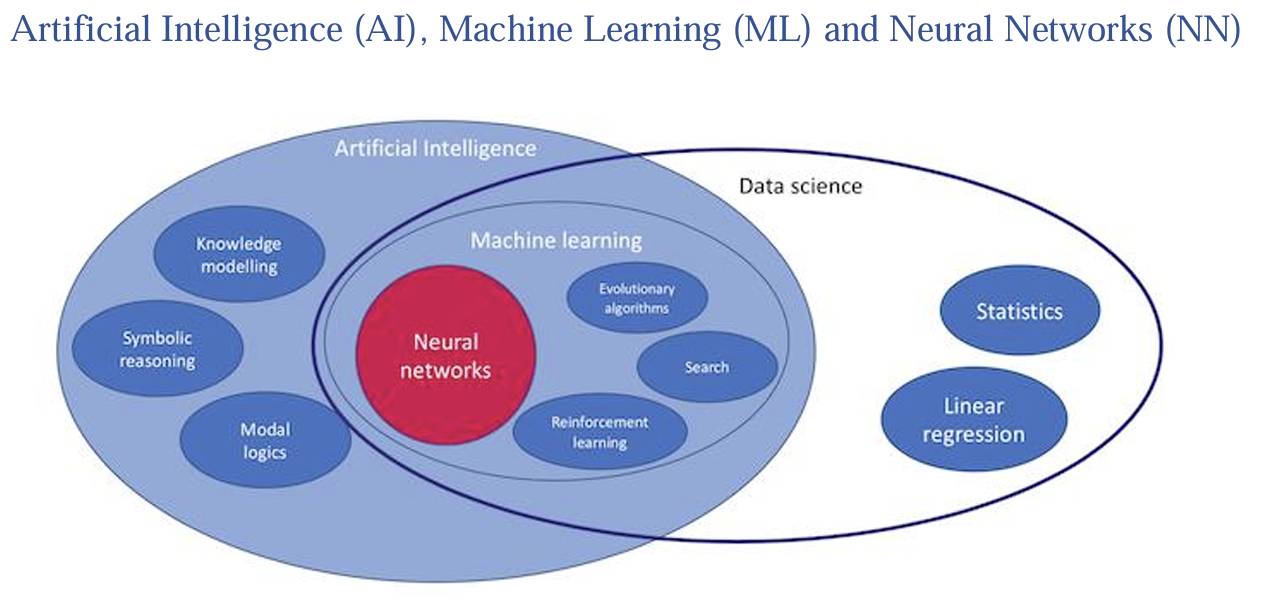
Figure 1: Visual Representation of Artificial Intelligence Domain
Artificial Intelligence (AI) is an extensive subject of computer science that focuses on building systems that can perform activities that normally require human intelligence. This include learning, solving problems, comprehending spoken language, and identifying patterns. Whereas Machine learning (ML) is a subset of the Artificial Intelligence which involves the development of algorithms using the data and make predictions out of it. ML models that can recognize patterns and make judgments with little to no human input are created using machine learning techniques. Neural Networks is special class of machine learning algorithm inspired by the structure of the human brain. With the use of layered nodes (neurons) provide an output based on the input data. NNs work especially well for applications like speech and picture recognition, natural language processing, and gaming. All the algorithms, be it neural networks or simple/complex machine learning are used to create/develop an AI application\(^{[1]}\)
Objective
This project’s main goal is to use neural networks to estimate the 2D incompressible Boussinesq equations. These equations describe the motion of buoyancy-driven fluid flows and are represented by the set of partial differential equations (PDEs)\(^{[2]}\):
\[\left\{\begin{array}{c} \partial_t u+u \cdot \nabla u+\nabla \mathrm{P}=v_x \partial_{x x} u+v_y \partial_{y y} u+\theta e_2 \\ \partial_t \theta+u \cdot \nabla \theta=k_{x x} \partial_{x x} \theta+k_{y y} \partial_{y y} \theta \\ \nabla \cdot \mathrm{u}=0 \end{array}\right.\]Where,\(x = (x,y) Χ = (𝑥,𝑦) \in R^2, t > 0\) and \(u = (u,v)^T, P, \theta\) denote, respectively, the velocity, pressure and buoyancy fields. The vertical unit vector \(e_2 = (0,1)^T\) and \(v_x, v_y, k_x, k_y\) are the viscosity and buoyancy diffusion coefficients respectively. The above equations can be simplified to the following for a partially dissipative system with a negligible thermal diffusion and when \(v_x, v_y = v\).
- X-momentum Equation:
- Y-momentum Equation:
- Continuity Equation:
- Advection Equation:
where,
- \(u\) is the velocity of fluid in x-direction,
- \(v\) is the velocity of fluid in y-direction,
- \(p\) is the pressure of the fluid,
- \(\theta\) is the temperature,
- \((x,y) \in 𝑅^2\) and
- \(t\) is the time
This project signifies the integration of Neural Networks and the laws of physics. This approach reduces the computational costs and improves the accuracy for higher dimension complex fluid dynamics problems when compared to traditional finite element methods\(^{[3]}\). The scope of this project extends the use of neural network models to approximate the solutions for higher dimension non-linear partial differential equations with different hyper-parameters.
Literature Review
McCulloch et.al in 1943, introduced the concept of deep learning, a subdivision of machine learning by explaining the working structure of biological neurons with a simple neural network using electrical circuits being active or inactive\(^{[4]}\). Deep learning, a subclass of machine learning, uses many-layered neural networks—hence the term “deep” Large volumes of data can be modelled by these deep neural networks (DNNs) to represent intricate patterns.
Frank Rosenblatt in 1958, using the brain cell activity from Hebb’s model, created the first feed forward layered neural network model in an IBM 704 machine for image recognition. The machine built with a single input and single output layer, after multiple trials learned to distinguish between left and right marked cards\(^{[5]}\). Ivakhnenko et.al, in 1967 published the work of a feed-forward multi-layered perceptron\(^{[6]}\).
Rumelhart et.al, in 1986 published a paper on backpropagation. The study outlines a number of neural networks where backpropagation operates significantly more quickly than in previous learning methodologies, enabling neural networks to be used to tackle problems that were previously thought to be intractable. The backpropagation method is currently the mainstay of neural network learning\(^{[7]}\). NNs are trained by a process called backpropagation, in which the model uses the chain rule to determine the gradient of the loss function with respect to each weight and then modifies the weights in order to minimize the loss.
Maizar Raissi et.al, in 2017 introduced the concept of Physics Informed Neural Networks (PINNs). These networks are trained to solve and approximate the solution of a nonlinear partial differential equations by also governing the laws of physics\(^{[8]}\). PINNs train neural networks using physical laws that are outlined by PDEs. PINNs use the problem’s known physics, encoded in PDEs, to direct learning rather than just depending on data. In scientific computing, this method works especially well for tackling forward and inverse issues.
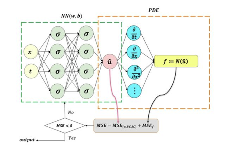
Figure 2: Working architecture of Physics Informed Neural Networks (PINNs)
Based on Fig.2, it can be understood that PINNs uses a feed-forward neural network with inputs as the known variables and generates a NN model to predict the output by also respecting the governing boundary conditions. PINNs uses automatic differentiation to calculate the differential operators and the loss functions of the PDE and the boundary conditions are calculated in the forward pass. During the backward pass, the weights and biases of the model are optimized using SCG, Adam, L-BFGS etc., to reduce the loss functions. The loss function can be calculated using a simple technique such as Mean Squared Error (MSE). Once the loss meets the criteria of being lower than a specific tolerance, the iterations are stopped and the optimized NN model is used to predict the outputs.
Lu Lu et.al, in 2020 created DeepXDE, an open-source python library and presented a paper showing the approximation theory, and error analysis of the physics-informed neural networks (PINNs) for solving different types of partial differential equations (PDEs)\(^{[9]}\).
Methodology
The project is carried out in different stages:
- Formulation of PDE
- Creating the domain and the spatial-temporal geometry
- Generating the data for training using random sampling and another data using uniformly spaced points
- Defining the neural network
- Compiling, Training and Validating the NN model
- Predicting the output using the final model and visualization of the data.
Unlike regular inputs for NN model, in PINNs, the co-ordinates \((𝑥,𝑦,𝑡) \in 𝑅^2\) inside the domain are the input data and the output of the model approximates the unknown values in the Boussinesq equations \(𝑢,𝑣,𝑝, \theta =𝐹(𝑥,𝑦,𝑡)\).
Partial Differential Equations The Boussinesq equations (1.1) are
\[\begin{gathered} \frac{\partial u}{\partial t}+u \frac{\partial u}{\partial x}+v \cdot \frac{\partial u}{\partial y}+\frac{\partial P}{\partial x}-v\left(\frac{\partial^2 u}{\partial x^2}+\frac{\partial^2 u}{\partial y^2}\right)=0 \\ \frac{\partial v}{\partial t}+u \frac{\partial v}{\partial x}+v \cdot \frac{\partial v}{\partial y}+\frac{\partial P}{\partial x}-v\left(\frac{\partial^2 v}{\partial x^2}+\frac{\partial^2 v}{\partial y^2}\right)=0 \\ \frac{\partial u}{\partial x}+\frac{\partial v}{\partial y}=0 \\ \frac{\partial \theta}{\partial t}+u \cdot \frac{\partial \theta}{\partial x}+v \cdot \frac{\partial \theta}{\partial y}=0 \end{gathered}\]Boundary Conditions
As mentioned earlier, this project focuses on solving the PDE using a new numerical method PINNs. The boundary and initial conditions in used to solve the Boussinesq equations is no-slip boundary condition on the walls using the Dirichlet boundary condition, and
\[\begin{gathered} 𝑢_0(𝑥,𝑦) = 𝑠𝑖𝑛(2\pi𝑦) 𝑠𝑖𝑛2(\pi𝑥)\\ 𝑣_0(𝑥,𝑦) = − 𝑠𝑖𝑛(2\pi𝑥) 𝑠𝑖𝑛2(\pi𝑦)\\ 𝜃_0 = 𝑠𝑖𝑛(3𝑥) 𝑐𝑜𝑠(2𝑦) + (𝑥−0.5)3 + 1/(𝑦+10) \end{gathered}\]as the initial conditions at time \(t=0\). The kinematic viscosity \((𝜈)\) is assumed to be 1.
Geometry and Domain
The geometry of the domain is defined as a rectangle for the spatial domain \([-1,1] \times [-1,1]\). As for the time domain, it varies from \(t=0\) to \(t=100\). The spatial and time domain are integrated to form the spatial-temporal domain used in PINNs to define the data points.
Implementation
Software and Libraries
NN open-source frameworks in python such as TensorFlow (developed by Google) and PyTorch (developed by Facebook) are used in this project to define the neural network model. These tools are helpful in building, training and deploying a deep learning model competently. For implementation of PINNs, the python library DeepXDE is used. DeepXDE uses TensorFlow, PyTorch, PaddlePaddle and JAX as backends to build and train the neural network. The geometry, PDE and the boundary conditions (BC & IC) are defined using the DeepXDE framework. For this project, TensorFlow is used as the backend of DeepXDE as it has the highest computational speed and supports most of the features for solving the Boussinesq equations. DeepXDE can also automatically choose the GPU as the main device for computation when TensorFlow is chosen as the backend. Other dependencies used by DeepXDE are Numpy, Matplotlib, SciPy, Scikit-Learn and Scikit-Optimize.
Multiple interactive development environments of Python such as Anaconda, Jupyter Lab and Google Colab are used in this project to write the code and the final code is submitted as a job file in a High-Performance Computing Cluster (HPCC) provided by the Institute for Cyber-Enabled Research (ICER). For computational research, scholars from industry and academia can use cyberinfrastructure provided by ICER. Multidisciplinary research in all areas of computational sciences is supported by ICER\(^{[10]}\).
Data Generation
Two main methods are used to generate the training data which provides two different models. The training data for the first model is generated with a random sampling using Latin Hypercube Sampling (LHS). A statistical technique for producing parameter values that guarantees thorough coverage of the parameter space is called Latin Hypercube Sampling (LHS). In order to avoid clustering and guarantee uniform exploration, it splits the range of each parameter into equally likely intervals and samples each interval exactly once. Because LHS requires fewer sample points for the same accuracy as simple random sampling, it is more efficient. It is versatile, applicable to a wide range of dimensions and distributions, and offers consistent coverage across multidimensional areas\(^{[11]}\).
For the latter model, the training data is generated in such a way that each point in the spatial temporal domain is uniformly distributed with equal spacing. The total number of quadrature training points using LHS are 25k and the second model with uniformly spaced training points are 25k.
Model Architecture
For this project, a neural network architecture with multiple important components was created. Three inputs, \(x, y,\) and \(t,\) which stand for the spatial and temporal coordinates, are received by the input layer. Four hidden layers with a total of 80 neurons each are used in this network. To account for the non-linearity in the model, the activation function hyperbolic tangent function (tanh) is used, and the output layer provides 4 outputs \(u,v,P\) and \(T\) corresponding to the velocity components, pressure, and temperature, respectively. The neural networks weights are initialized using the Xavier normal initialization method (Glorot normal) to maintain the variance of the activations and gradients across the layers of the network, which helps to avoid the vanishing or exploding gradient problems during training.
The model training begins using the Adam optimizer with a learning rate of \(1e-3\) and 20000 iterations. When the model reaches a good approximation using Adam, then it is refined using the L-BFGS optimizer with the maximum number of iterations set at 3000. L-BFGS is a quasi-Newton method that is particularly effective for optimizing differentiable functions, which helps in achieving a more precise and stable solution.
Training and Validation
To make sure that the model follows the physical principles outlined by the governing equations as well as the underlying patterns in the data, the training procedure is carefully designed. The Adam optimizer is initially used to train the model. The learning rate is constantly adjusted throughout this phase using a learning rate schedule, which improves optimizer efficiency and helps avoid problems like under- or overfitting. The L-BFGS optimizer is used to refine the model after the initial training. This is an important step since L-BFGS offers better convergence properties for model fine-tuning.
The model’s performance is assessed using a wide range of metrics and techniques. In order to guarantee that the model’s predictions satisfy the physical laws, the loss function is constructed to incorporate the residuals of the partial differential equations (PDEs). Comparing the expected and actual values at different domain points is the process of validation. This comparison is necessary to evaluate the model’s correctness and make sure it applies well to data that hasn’t been seen before.
Results and Conclusion
The initial conditions used for training the model are visualized in Fig.3,
\[\begin{gathered} T(𝜃). 𝑢0(𝑥, 𝑦) = 𝑠𝑖𝑛(2𝜋𝑦)𝑠𝑖𝑛2(𝜋𝑥) \\ 𝑣0(𝑥,𝑦) = − 𝑠𝑖𝑛(2𝜋𝑥)𝑠𝑖𝑛2(𝜋𝑦) \\ 𝜃_0 = 𝑠𝑖𝑛(3𝑥) 𝑐𝑜𝑠(2𝑦) + (𝑥 − 0.5)3 + 1/(𝑦 + 10) \end{gathered}\]and Fig.4 illustrates the domain of two different models with Latin hypercube sampling and uniformly spaced sampling. The total number of training points used for network including PDE and BC training points are 25k in each of the two models.
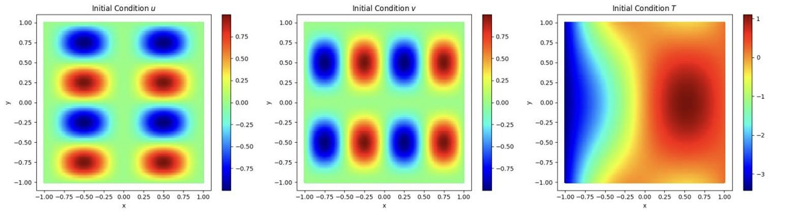
Figure 3: Initial Conditions for Velocity Components u,v and Temperature T
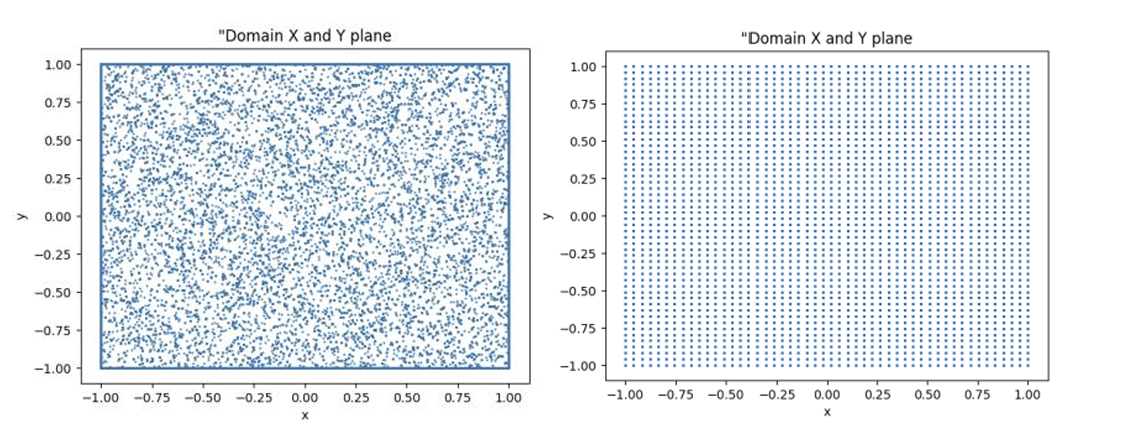
Figure 4: Training data generated using, Left – Random Sampling technique, Right – Uniform sampling distribution
| Model | Sampling | Total Training Points | PDE points | BC points | Learning Rate | Total Loss |
|---|---|---|---|---|---|---|
| 1 | LHS | 25000 | 10000 | 15000 | 1.0E-3 | 1.4E-4 |
| 2 | Uniform | 25340 | 18000 | 7340 | 1.0E-3 | 2.27 |
Table 1: Model comparison of LHS and Uniform sampling
After training the model with 20000 iterations using Adam optimizer and then refining it using L-BFGS optimizer, the total loss values for the first model is \(1.4e-4\) and for the second model is \(2.27e+0\). As DeepXDE uses its own sampling stratification for the distribution of training points, there is a lot of difference between the training points for the PDEs and the boundary conditions in both the models. Although, the total training points are almost same, the loss for model 1 as it was able to handle the noisy data.
For model 1, the training and test loss become less than \(1e-3\) after 2500 iterations. As per model 2, the loss values although high come to a constant value after 1000 iterations. From this, we can conclude that, the number of iterations for the model does not effect the losses directly. Instead, it is the number of sampling points and its distribution.
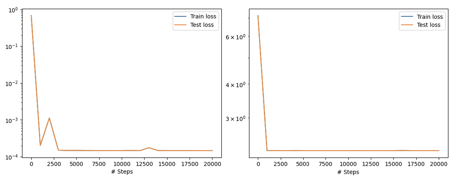
Figure 5: Training and test losses for both Model 1 (Left) and Model 2 (Right) for a total of 20000 iterations and refining with the L-BFGS.
Fig.6, shows the visualized distribution of temperature plots after using model 1 to approximate the solutions for the Boussinesq equations. It is quite surprising that even with a very low training loss of \(1.4e-4\), model 1 is still not able to predict the temperature plots properly. It can be seen that at time \(t=0\), the temperature plot does not match with the initial plot of temperature at \(t=0\) (Fig.3). It can also be observed that after a certain time, the temperature distribution slowly comes to a state of equilibrium.
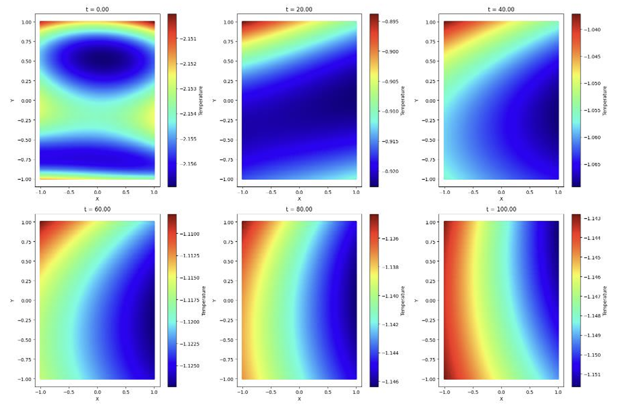
Figure 6: Temperature Distribution plots predicted using Model 1
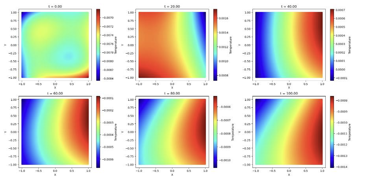
Figure 7: Temperature Distribution plots predicted using Model 2
When used model 2, with higher loss compared to model 1 to predict the solutions of the Boussinesq equations, the temperature plots are entirely different. This was quite expected as the loss value was very high for model 2. Although, model 1 has better loss, it was still not predicted the value properly. As the exact solution for the Boussinesq equation is not known due to its high non-linearity nature, it cannot be confirmed if the predictions using model 1 are entirely incorrect.
Future Scope
The models can be further optimized by changing the hyperparameters such as the learning rate, number of training points and the number of iterations. To decrease the computational time, the number of training points for the boundary and initial conditions used was less, which probably resulted in the incorrect approximation of the equations. By using the GPU sources of the HPCC provided by ICER, the computational time can be further increased even at higher sample points. This can be strongly backed as the study was initially started with only 5000 sample points and the loss values decreased as the number of sample points increased. Further study is continued on updating the boundary conditions to a no-penetration and a zero vorticity boundary conditions to approximate the Boussinesq equations with a greater number of sample points and also using the GPU resources. The updated models with the new boundary conditions and initial conditions will be compared with the results of the traditional methods\(^{[1]}\) for the computational time and accuracy.
References
[1] Sieuwert van Otterloo. AI, Machine Learning and neural networks explained
[2] Charles R. Doering, Jiahong Wu, Kun Zhao, Xiaoming Zheng, Long time behavior of the two dimensional Boussinesq equations without buoyancy diffusion, Physica D: Nonlinear Phenomena, Volumes 376–377, 2018, Pages 144-159, ISSN 0167-2789, https://doi.org/10.1016/j.physd.2017.12.013.
[3] Tamara G Grossmann, Urszula Julia Komorowska, Jonas Latz, Carola-Bibiane Schönlieb, Can physics informed neural networks beat the finite element method?, IMA Journal of Applied Mathematics, Volume 89, Issue 1, January 2024, Pages 143–174, https://doi.org/10.1093/imamat/hxae011
[4] McCulloch, W.S., Pitts, W. A logical calculus of the ideas immanent in nervous activity. Bulletin of Mathematical Biophysics 5, 115–133 (1943). https://doi.org/10.1007/BF02478259
[5] Rosenblatt, F. (1958). The perceptron: A probabilistic model for information storage and organization in the brain. Psychological Review, 65(6), 386–408. https://doi.org/10.1037/h0042519
[6] Ivakhnenko, A.G., Lapa, V.G., & Mcdonough, R.N. (1967). Cybernetics and forecasting techniques.
[7] Rumelhart, D., Hinton, G. & Williams, R. Learning representations by back-propagating errors. Nature 323, 533–536 (1986). https://doi.org/10.1038/323533a0
[8] Raissi, Maziar; Perdikaris, Paris; Karniadakis, George Em (2017-11-28). “Physics Informed Deep Learning (Part I): Data-driven Solutions of Nonlinear Partial Differential Equations”. https://doi.org/10.48550/arXiv.1711.10561 Solving
[9] Lu Lu, Xuhui Meng, Zhiping Mao, and George Em Karniadakis. DeepXDE: A Deep Learning Library for Differential https://doi.org/10.1137/19M1274067 Equations. SIAM
[10] Institute for Cyber-Enabled Research (ICER). https://icer.msu.edu/ Review 2021 63:1, 208-228.
[11] McKay, M. D., Beckman, R. J., & Conover, W. J. (1979). A Comparison of Three Methods for Selecting Values of Input Variables in the Analysis of Output from a Computer Code. Technometrics, 21(2), 239–245. https://doi.org/10.2307/1268522
[12] Tim De Ryck, Ameya D Jagtap, Siddhartha Mishra, Error estimates for physics-informed neural networks approximating the Navier–Stokes equations, IMA Journal of Numerical Analysis, Volume 44, Issue 1, January 2024, Pages 83–119, https://doi.org/10.1093/imanum/drac085