Objective: -

In this problem, we will write a Cantera code to calculate the Auto Ignition time for Methane under various conditions. This problem is divided into two parts.

Part 1: -

Simulate the Auto Ignition Time for Methane under the following conditions, (simulation time = 10 secs)

• Plot the variation of Auto Ignition time of Methane with a constant temperature of 1250K and pressure varying from 1 to 5 atm.
• Plot the variation of Auto Ignition time of Methane with a constant pressure of 5 atm and temperature varying from 950K to 1450K.

Part 2: -

Further, observe and print the rate of change of molar concentrations of the given elements \((H_2O, O_2,\) and \(OH)\) with respect to the time, (simulation time = 10 secs)

Explain the behaviour of the graph for 2 cases,

• When Temperature is 1000K and pressure 5 bar
• When Temperature is 500K and pressure 5 bar

Solution: -

Part 1: -

In the first part, we are going to simulate and show the variation of Auto Ignition time of Methane combustion with respect to given pressure and temperature parameters using the cantera module of python.

For both of the cases, we are considering an Ideal gas reactor and its corresponding Reactor Network. The simulation time given for these cases is about 10 seconds. Auto Ignition time is the time when the temperature of the reactor is Initial Temperature plus 400K. The Auto Ignition time is very small, occurring in milli seconds.

Case 1: -

In this case, we are going to plot the variation of Auto Ignition of Methane with a constant temperature of 1250 Kelvin and pressure varying from 1 to 5 atmospheres. We are considering and arranging five pressure values for this case.

The python code for the above case is given below: -

import sys
import numpy as np 
import cantera as ct 
import matplotlib.pyplot as plt 


gas = ct.Solution('gri30.xml')
T_start = 950
T_end = 1450
P = 5*101325

sim_time = 10*1000  # Simuation Time--> 10 seconds

n = 10
temp = np.linspace(T_start,T_end,n)
Ignition_delay = []

for T in temp:
	gas.TPX = T, P, {'CH4':1, 'O2':2, 'N2':7.52}

	r = ct.IdealGasReactor(gas) # Reactor
	sim = ct.ReactorNet([r]) # Reactor Network

	time = 0.0 # Initial Time

	# States of Reactor---> attribiutes of the reactor
	states = ct.SolutionArray(gas, extra = ['t_ms','t']) 

	T_old = T

	i = 1
	for i in range(sim_time+1):
		time += 1e-03

		sim.advance(time) # Advancing the reactor w.r.t the time step

		states.append(r.thermo.state, t_ms = time*1e3, t = time)

		T_new = states.T
		T_new = T_new[i-1]

		if ((T_new - T_old)>=400):

			Ignition_delay.append(time)

		T_old = states.T
		T_old = T_old[i-1]

	plt.subplot(2,1,1)
	plt.plot(states.t_ms, states.T)

plt.legend(['T_start = ' + str(T) + '[K]' for T in temp])
plt.xlabel('Time [ms]')
plt.ylabel('Temperature [K]')

plt.subplot(2,1,2)
plt.plot(temp, Ignition_delay, '-o')
plt.xlabel('Initial Temperature [K]')
plt.ylabel('Ignition Delay [ms]')

print('Ignition Delay = ', Ignition_delay)
print('Temperature = ', temp)
plt.show()

Case 2: -

For this case, we are going to plot the variation of Auto Ignition of Methane with a constant pressure of 5 atmospheres and temperature varying from 950 kelvin to 1450 kelvin. Similar to the previous case, we are considering and arranging five temperature values for this case.

The python code for the above case is given below: -

import sys
import numpy as np 
import cantera as ct 
import matplotlib.pyplot as plt 

gas = ct.Solution('gri30.xml')

T = 1250
P_start = 101325
P_end = 5*101325

sim_time = 10*1000  #10 seconds

n = 8 # Number of values for pressure
press = np.linspace(P_start,P_end,n)
Ignition_delay = []

for P in press:

	gas.TPX = T, P, {'CH4':1, 'O2':2, 'N2':7.52}
	r = ct.IdealGasReactor(gas) # Reactor
	sim = ct.ReactorNet([r]) # Reactor Network

	time = 0.0 # Initial Time

	# States of Reactor which include all attribiutes of the reactor
	states = ct.SolutionArray(gas, extra = ['t_ms','t'])

	T_old = T

	i = 1
	for i in range(sim_time+1):
		time += 1e-03

		sim.advance(time) # Advancing the reactor w.r.t the time step

		states.append(r.thermo.state, t_ms = time*1e3, t = time)

		T_new = states.T
		T_new = T_new[i-1]

		if ((T_new - T_old)>=400):
			Ignition_delay.append(time)

		T_old = states.T
		T_old = T_old[i-1]

	plt.subplot(2,1,1)
	plt.plot(states.t_ms, states.T)

plt.legend(['P_start = ' + str(P/101325) + '[atm]' for P in press])
plt.xlabel('Time [ms]')
plt.ylabel('Temperature [K]')

plt.subplot(2,1,2)
plt.plot(press/101325, Ignition_delay, '-o')
plt.xlabel('Initial Pressure [Pa]')
plt.ylabel('Ignition Delay [ms]')

print('Ignition Delay = ', Ignition_delay)
print('Pressure = ', press)
plt.show()

Results and Observations: -

Case 1: -

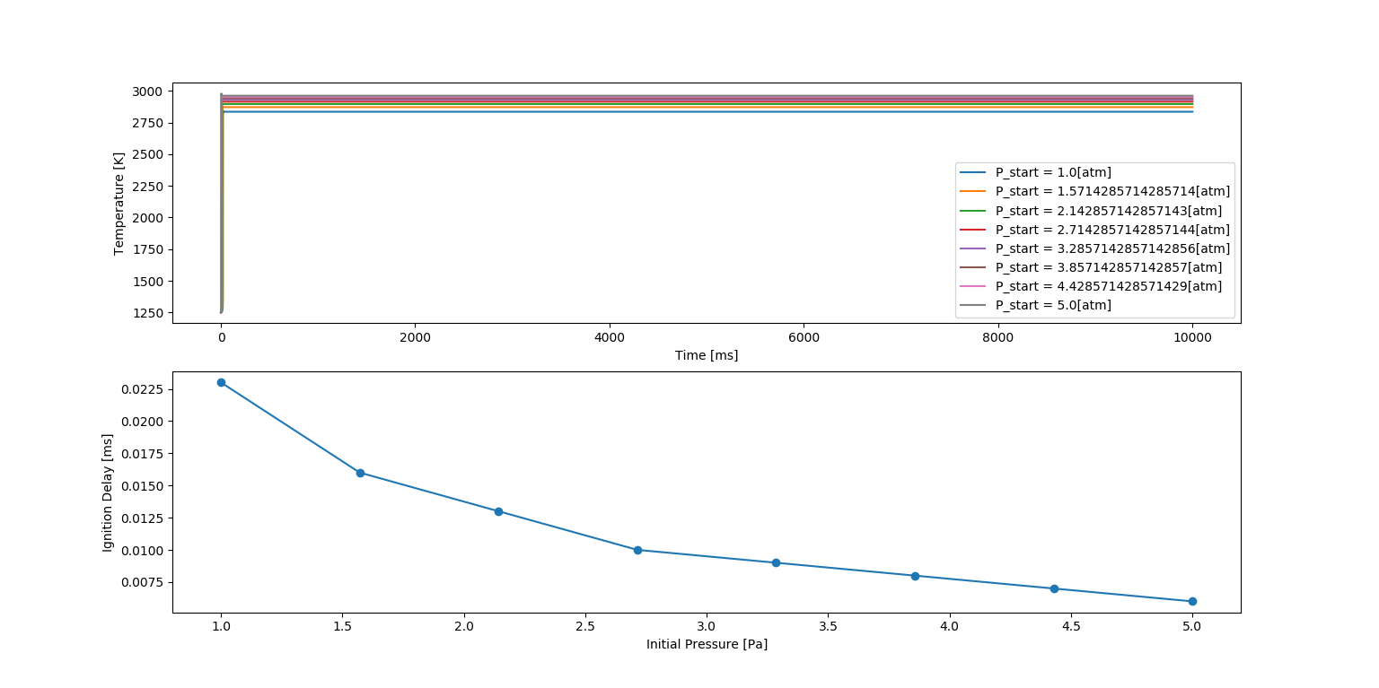
Auto Ignition time plot of Methane with a constant temperature of 1250K and pressure varying from 1 to 5 atm.

Auto Ignition Part 1 - Case 1

Ignition Delay with Temperature Variation

In the above figure, there are two plots. The top plot shows the Auto Ignition of Methane with eight varying pressures which can be seen in the legend. The auto ignition is occurring approximately in the range of 0 to 25 milli seconds for the given temperature range.

The bottom plot shows the Ignition delay with respect to the pressure values taken. We can clearly see that the Ignition Delay is decreasing as the pressure increases. This infers that Ignition delay is sensitive to pressure.

Case 2: -

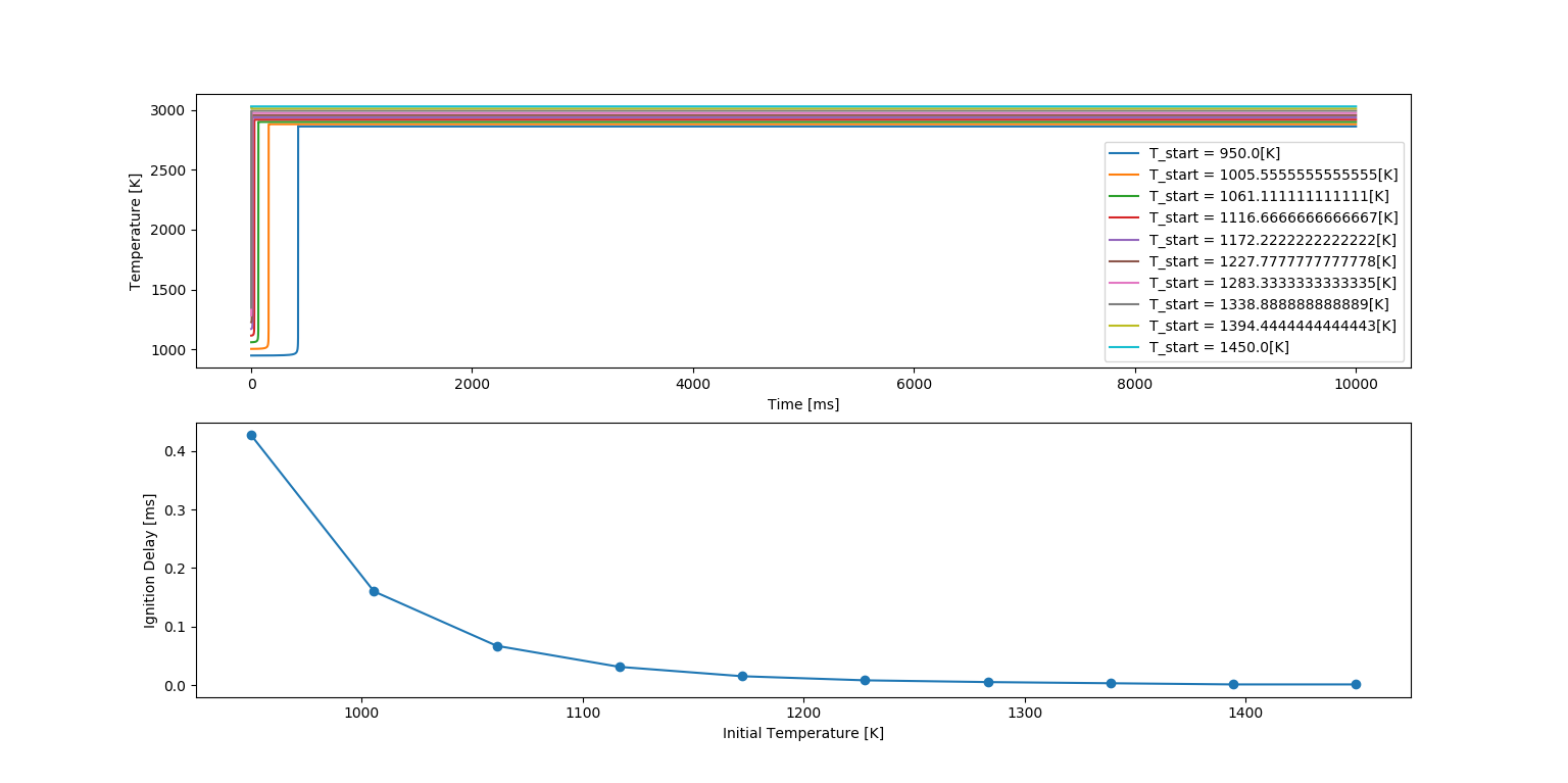
Auto Ignition time plot of Methane with a constant pressure of 5 atm and temperature varying from 950K to 1450K.

Auto Ignition Part 1 - Case 2

Ignition Delay with Temperature Variation

Similarly, in this figure, the top plot shows the Auto Ignition of Methane with ten varying temperatures which can be seen in the legend. The auto ignition is occurring approximately in the range of 0 to 55 milli seconds for the given pressure range.

The bottom plot shows the Ignition delay with respect to the temperature values taken. We can clearly see that the Ignition Delay is decreasing as the temperature increases. But in this plot, we observe that the Ignition delay is decreasing way faster when compared to pressure. This is obvious because, as the temperature increases, the auto ignition is occurring very fast. This infers that Ignition delay is sensitive to temperature.

Inference: -

The following are the conclusions we have gathered from the above results: -

• The Ignition Delay plot shows that the Ignition Delay is exponential.
• Ignition Delay is sensitive to both pressure and temperature showing that the combustion is occuring quickly when these parameters are increasing.
• Ignition Delay is more sensitive to temperature.

Part 2: -

In this part of the challenge, we are going to observe the rate of change of molar concentrations of the given elements “H2O, O2, OH” with respect to the simulation time using cantera module of python.

For this part of the challenge, we have two cases where we will be observing the rate of change of molar concentrations of the given elements when the pressure is at five bar and temperature at 1000 kelvin and 500 kelvin for a methane combustion. The given simulation time is 10 seconds.

The python code for the above problem is given below: -

# Code to observe the rate of change of molar concentrations of the given elements "H2O, O2, OH" with respect to the time 10 seconds
# CH4 + 2(O2 + 3.76N2) = CO2 + 2H20 + 7.52N2
#states.X[:,gas.species_index('species')])

import sys
import numpy as np 
import cantera as ct 
import matplotlib.pyplot as plt 

gas = ct.Solution('gri30.xml')

temp = [1000, 500]
P = 5*101325

incre = 10e-3
end_time = 10 #in seconds

sim_time = end_time/incre 

species = {'CH4':1, 'O2':2, 'N2':7.52}

for T in temp:
	gas.TPX = T, P, species
	r = ct.IdealGasReactor(gas) # Reactor
	sim = ct.ReactorNet([r]) # Reactor Network

	time = 0.0 # Initial Time

	states = ct.SolutionArray(gas, extra = ['t_ms','t']) # States of Reactor---> attribiutes of the reactor

	for n in range(int(sim_time)):
		time += incre

		sim.advance(time) # Advancing the reactor w.r.t the time step

		states.append(r.thermo.state, t_ms = time*1e3, t = time)

	plt.subplot(1,3,1)
	plt.plot(states.t, states.X[:,gas.species_index('H2O')])
	plt.xlabel('Time [s]')
	plt.ylabel('H2O Mole Fraction')

	plt.subplot(1,3,2)
	plt.plot(states.t, states.X[:,gas.species_index('O2')])
	plt.suptitle('Rate of Change of H2O, O2, OH Molar Concentration at '+str(T)+' Kelvin')
	plt.xlabel('Time [s]')
	plt.ylabel('O2 Mole Fraction')
	
	plt.subplot(1,3,3)
	plt.plot(states.t, states.X[:,gas.species_index('OH')])
	plt.xlabel('Time [s]')
	plt.ylabel('OH Mole Fraction')

	plt.show()

Results and Observations: -

Case 1: -

Auto Ignition Part 2 - Case 1

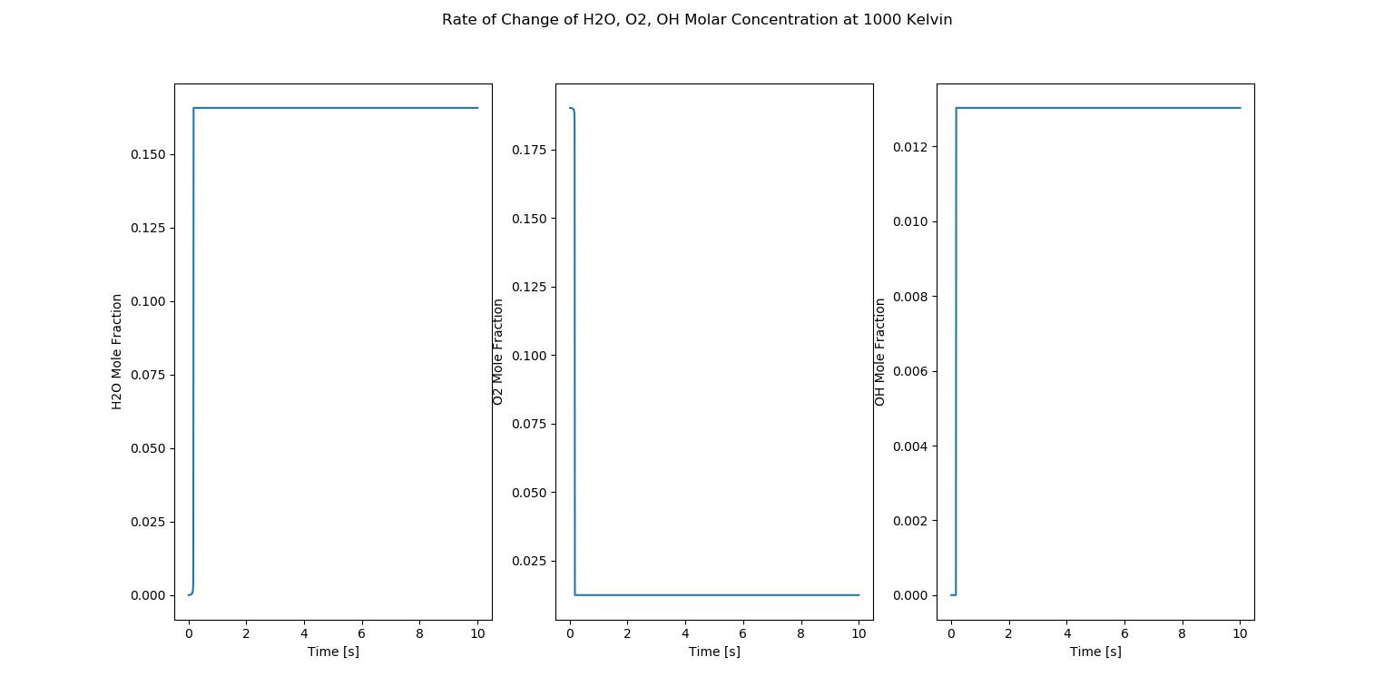
Molar Concentrations

In the above figure, we observe three plots which are show the rate of change of \(H_2O, O_2, OH\) molar fractions at 1000 kelvin.

The first plot shows that the mole fraction of \(H_2O\) is very less before the Auto Ignition takes place and increases and stabilizes. As discussed earlier, this is a methane combustion. In the combustion reaction, \(H_2O\) is the product which is forming. The plot shows that \(H_2O\) is being formed and increasing as the combustion is occurring. The second plot shows the O2 mole fraction is decreasing. This trend is occurring because, in the combustion reaction, \(O_2\) is a reactant as it is the oxidizer for combustion. As the combustion process takes place, the \(O_2\) is being used and its mole fraction is decreasing respectively.

Similar to the first lot, \(OH\) is also a product of the methane combustion reaction. As the combustion reaction is occurring, the \(OH\) is being used which can be seen as it’s mole fraction is increasing in the third plot. But it is to be noted that \(OH\) is an additional species which is being formed in the reaction and is not generally depicted in a methane reaction mechanism.

Case 2: -

Auto Ignition Part 2 - Case 2

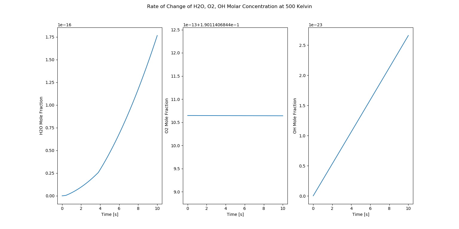
Molar Concentrations

In the above figure, we observe three plots which are show the rate of change of \(H_2O, O_2, OH\) molar fractions at 500 kelvin.

At an initial glance, it is hard to understand what is occuring in the plots. But first, we have to understand that at 500 kelvin methane cannot combust because the auto ignition temperature of methane is around 600 celsius which is around 873.15 kelvin. This value is way higher than our temperaure consideration. So, we can establish that combustion is not occuring in this case.

Yet, we observe changes in the mole fractions of \(H_2O\) and \(OH\) while \(O_2\) mole fraction is constant. This is occurring because \(H_2O\) and \(OH\) have single bonds and the energy of the reactor at 500 kelvin is enough to break the bonds. And in the case of \(O_2\), there is no change as \(O_2\) has double bonds and it takes more amount of energy to break its bonds when compared to the single bonds of \(H_2O\) and \(OH\). This kind of phenomenon is happening because of the ambient reactions occurring in the reactor. If we decrease the temperature more, this phenomenon will not occur as there is no sufficient energy to break the bonds of \(H_2O\) and \(OH\).

If you are interested, you can check out the project code here. And if you have any questions, you can always reach out to me!