
2D Shock-Vortex Interaction
Published:
Problem Statement
In this work, we are going to explore the Rusanov and MacCormack schemes in 2D for shock-vortex interactions. In this work we explored the Euler equations in the case of a one-dimensional shock tube. For low Mach number flows, the exact solution to the current problem is where the vortex shifts by distances, \(\Delta x = u_{\infty}\) and \(\Delta y = v_{\infty}\), where \(u_{\infty}\) and \(v_{\infty}\) are far-field velocities.
Method of Solution
We will initialize the velocity and temperature as:
\[( u = u_\infty - Ma_c \cdot a_c \cdot y \cdot \exp\left[\frac{(1 - (r^*)^2)}{2}\right] )\] \[( v = v_\infty - Ma_c \cdot a_c \cdot x \cdot \exp\left[\frac{(1 - (r^*)^2)}{2}\right] )\] \[( T = 1 - \frac{\gamma - 1}{2} \cdot Ma_c^2 \left(1 + \frac{\gamma - 1}{2} \cdot Ma_c^2 (r^*)^2 \exp(1 - (r^*)^2)\right) )\]Where:
- \(L = 1 \, \text{m}\),
- \(R_c = L/10\),
- \(x_c = L/2\),
- \(y_c = L/2\) and
- \(Ma_c = 0.3\).
The vortex is subject to a shock wave initialized at \(( x_c = L/4 )\), using the Riemann benchmark.
Initial Conditions
The initial conditions for the shock-vortex problem are summarized below:
| Test | \(\rho_L\) | \(u_L\) | \(p_L\) | \(\rho_R\) | \(u_R\) | \(p_R\) | Wave L | Wave R | Description |
|---|---|---|---|---|---|---|---|---|---|
| 1 | 1.0 | 0.0 | 1.0 | 0.125 | 0.0 | 0.1 | R | S | Sod problem |
Table 1: Summary of shock initial conditions for Riemann Test 1.
| \(x\) | \(\rho\) | \(p\) | \(u\) | \(v\) |
|---|---|---|---|---|
| \(\leq x_s\) | \(\rho_L\) | \(p_L\) | \(u_L\) | 0 |
Table 2: Summary of initial conditions for \(( x \leq x_s )\) and \(( x > x_s )\)
We are going to explore the use of 2D code to solve the shock-vortex problem on an \(((L, L))\) grid with Neumann flux conditions in the x-direction and periodic boundaries in the y-direction. For all cases, we will solve the Euler equations using both MacCormack and Rusanov methods.
The 2D Euler equations are given as:
\[Q_t + F_x + G_y = 0\]Where:
\[Q_t = \begin{bmatrix} \rho \\ \rho u \\ \rho v \\ \rho e_t \\ \end{bmatrix}\]is the vector of conservative variables,
\[F_x = \begin{bmatrix} \rho u \\ \rho u^2 + p \\ \rho uv \\ \rho uH \\ \end{bmatrix}\]is the vector of fluxes in the x-direction, and
\[G_y = \begin{bmatrix} \rho v \\ \rho uv \\ \rho v^2 + p \\ \rho vH \\ \end{bmatrix}\]is the vector of fluxes in the y-direction.
Here,
\[e_t = e + \frac{(u^2 + v^2)}{2}\]is the total energy, and
\[H = h + \frac{(u^2 + v^2)}{2} = e + \frac{p}{\rho} + \frac{(u^2 + v^2)}{2}\]is the total enthalpy.
Numerical Methods
The above 2D Euler equations will be solved using two different methods outlined below through their discretized equations:
MacCormack Method (Finite Difference Formulation)
Predictor Step:
\[Q^{n+1}_{i,j} = Q^n_{i+1,j} - \frac{\Delta t}{\Delta x} (F^n_{i+1,j} - F^n_{i,j}) - \frac{\Delta t}{\Delta y} (G^n_{i,j+1} - G^n_{i,j})\]Corrector Step:
\[Q^{n+1}_{i,j} = \frac{1}{2} \left[ Q^n_{i,j} + Q^{n+1}_{i,j} \right] - \frac{\Delta t}{\Delta x} (F^{n+1}_{i,j} - F^{n+1}_{i-1,j}) - \frac{\Delta t}{\Delta y} (G^{n+1}_{i,j} - G^{n+1}_{i,j-1})\]To achieve all possible permutations to avoid biasing the solution, the predictor and corrector schemes are sequenced using forward and backward differencing.
Rusanov Method (Finite Volume Formulation)
\[Q^{n+1}_{i,j} = Q^n_{i,j} - \frac{\Delta t}{\Delta x} \left[ F^n_{i+1/2,j} - F^n_{i-1/2,j} \right] - \frac{\Delta t}{\Delta y} \left[ G^n_{i,j+1/2} - G^n_{i,j-1/2} \right]\]Where:
\[F^n_{i+1/2,j} = \frac{1}{2} \left( F^n_{i,j} + F^n_{i+1,j} \right) - \max \left[ |u|_{i,j} + a_{i,j}, |u|_{i+1,j} + a_{i+1,j} \right] (Q^n_{i+1,j} - Q^n_{i,j})\] \[G^n_{i,j+1/2} = \frac{1}{2} \left( G^n_{i,j} + G^n_{i,j+1} \right) - \max \left[ |u|_{i,j} + a_{i,j}, |u|_{i,j+1} + a_{i,j+1} \right] (Q^n_{i,j+1} - Q^n_{i,j})\]As a part of this work, different computer programs (refer to the Appendices) using Python have been developed to solve the Euler equations and explore the given methods.
Results
Baseline Shock Cases:

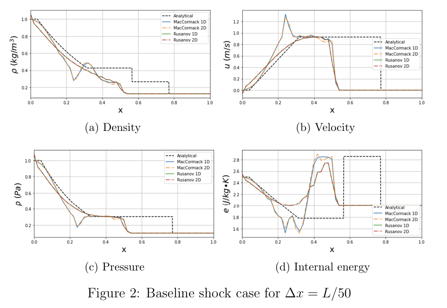
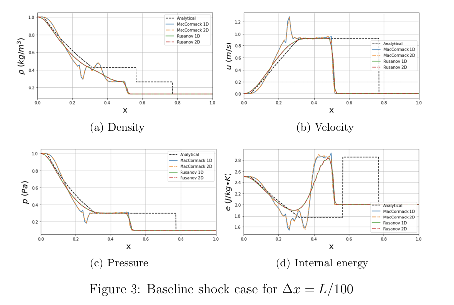
- MacCormack and Rusanov schemes were implemented at various grid resolutions using Python and compared their behavior with respect to 2D Isentropic vortex formation and shock-vortex interaction in low and high Mach numbers.
- Implemented and analyzed enstrophy, vorticity source terms (dilatation and baroclinic torque), and contour plots to visualize the vortex behavior.
- Demonstrated the superiority of the MacCormack solver over the Rusanov scheme for isentropic vortex formation and Shock-Vortex interaction.