
Comparative Study of RANS Models
Published:
Introduction
CFD simulations consist of understanding fluid flow under various effects and in different environments, these are accomplished by the Navier-Stokes equations which govern the physics behind the flows. These equations can describe any effects of different forces acting on a fluid and its resulting flow behavior. But, they cannot be solved in a closed form for every flow situation or system. To reduce the complexity of the simulations, certain numerical approaches were introduced, such as,
- Direct Numerical Simulations
- Large Eddy Simulations and
- Reynolds Averaged Numerical Simulations
The turbulence models which we are currently implementing in this scenario fall under the category of RANS (Reynolds Averaged Navier-Stokes) models or in terms of OpenFOAM RAS models. The RANS models are the most sought after in CFD for reducing the complexity of flows. These models are used to solve time averaged N-S equations for any turbulent length scales.
The following simulations for different turbulence models are performed using the 2D Backward facing step tutorial case in OpenFOAM. The following files show the case setup, and we will begin with the blockMeshDict file which defines the mesh.
Case Setup
This canonical case is based on the description by Driver and Seegmiller
D.M. Driver and H.L. Seegmiller. Features of a reattaching turbulent shear
layer in divergent channel flow. AIAA Journal, 23(2):163–171, 1985.
where the mesh is based on the Langley Research Center Turbulence Modeling Resource set-up provided at:
https://turbmodels.larc.nasa.gov/backstep_val.html
blockMeshDict
/*--------------------------------*- C++ -*----------------------------------*\
| =========                 |                                                 |
| \\      /  F ield         | OpenFOAM: The Open Source CFD Toolbox           |
|  \\    /   O peration     | Version:  v2112                                 |
|   \\  /    A nd           | Website:  www.openfoam.com                      |
|    \\/     M anipulation  |                                                 |
\*---------------------------------------------------------------------------*/
FoamFile
{
    version     2.0;
    format      ascii;
    class       dictionary;
    object      blockMeshDict;
}
// * * * * * * * * * * * * * * * * * * * * * * * * * * * * * * * * * * * * * //

scale   0.0127;

vertices
(
    ( -130   1   1) // 0
    ( -110   1   1) // 1
    (    0   1   1) // 2
    (    0   0   1) // 3
    (    8   0   1) // 4
    (   50   0   1) // 5
    (    8   1   1) // 6
    (   50 3.125 1) // 7
    (   50   9   1) // 8
    (    8   9   1) // 9
    (    0   9   1) // 10
    ( -110   9   1) // 11
    ( -130   9   1) // 12

    ( -130   1   0) // 13
    ( -110   1   0) // 14
    (    0   1   0) // 15
    (    0   0   0) // 16
    (    8   0   0) // 17
    (   50   0   0) // 18
    (    8   1   0) // 19
    (   50 3.125 0) // 20
    (   50   9   0) // 21
    (    8   9   0) // 22
    (    0   9   0) // 23
    ( -110   9   0) // 24
    ( -130   9   0) // 25
);


ySpacing ((0.3 0.47 250)(0.2 0.06 1)(0.3 0.47 0.004));
ySpacing2 ((0.75 0.3 1)(0.25 0.7 0.004));
yWall ((0.5 0.5 100)(0.5 0.5 0.03));

yLower1 ((0.4 0.7 50)(0.6 0.3 1));
yLower2 ((1 1 50));

//yUpper1 ((0.1 0.15 2)(0.75 0.35 4)(0.25 0.5 0.005));
yUpper1 ((0.1 0.2 2)(0.75 0.35 5)(0.25 0.45 0.005));

blocks
(
    // Coarse

    // Block 0
    hex (13 14 24 25 0 1 11 12)
    (15 20 1)
    simpleGrading (1 1 1)

    // Block 1
    hex (14 15 23 24 1 2 10 11)
    (88 20 1)
    simpleGrading (1 1 1)

    // Block 2
    hex (16 17 19 15 3 4 6 2)
    (20 10 1)
    simpleGrading (1 1 1)

    // Block 3
    hex (17 18 20 19 4 5 7 6)
    (60 10 1)
    simpleGrading (1 1 1)

    // Block 4
    hex (15 19 22 23 2 6 9 10)
    (20 20 1)
    simpleGrading (1 1 1)

    // Block 5
    hex (19 20 21 22 6 7 8 9)
    (60 20 1)
   simpleGrading (1 1 1)
);

edges
(
);

boundary
(

    inlet
    {
        type patch;
        faces
        (
            (13 0 12 25)
        );
    }
    outlet
    {
        type patch;
        faces
        (
            (18 20 7 5)
            (20 21 8 7)
        );
    }
    lowerWallStartup
    {
        type symmetryPlane;
        faces
        (
            (13 14 1 0)
        );
    }
    upperWallStartup
    {
        type symmetryPlane;
        faces
        (
            (25 12 11 24)
        );
    }
    upperWall
    {
        type wall;
        faces
        (
            (24 11 10 23)
            (23 10 9 22)
            (22 9 8 21)
        );
    }
    lowerWall
    {
        type wall;
        faces
        (
            (14 15 2 1)
            (15 2 3 16)
            (16 17 4 3)
            (17 18 5 4)
        );
    }
    front
    {
        type empty;
        faces
        (
            (0 1 11 12)
            (1 2 10 11)
            (3 4 6 2)
            (4 5 7 6)
            (2 6 9 10)
            (6 7 8 9)
        );
    }
    back
    {
        type empty;
        faces
        (
            (13 25 24 14)
            (14 24 23 15)
            (16 15 19 17)
            (17 19 20 18)
            (15 23 22 19)
            (19 22 21 20)
        );
    }

);

// ************************************************************************* //
The step height is 0.127 m or 1.27 cm. The length is taken from -110 to +50 (to be scaled to 0.0127 m). Simple grading is applied in the blocks. Compared to the previous test cases, the blockMeshDict here is formulated with respect to a turbulent nature case, which yields the specifications of y+ quantities and dimensions (ySpacing, yWall, yLower and yUpper).
The above setup yields the following mesh:
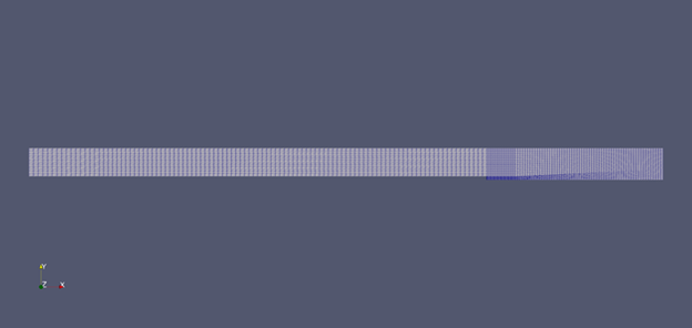
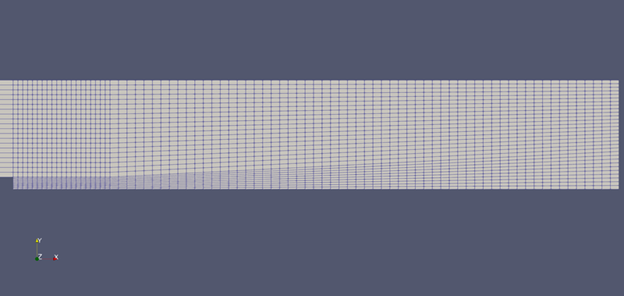
The mesh, particularly at the backward facing step, is as follows:
Velocity 0/U
For the velocity, we are initializing the inlet with a uniform velocity of 44.2 meters and the outlet as zero gradient.
/*--------------------------------*- C++ -*----------------------------------*\
| =========                 |                                                 |
| \\      /  F ield         | OpenFOAM: The Open Source CFD Toolbox           |
|  \\    /   O peration     | Version:  v2206                                 |
|   \\  /    A nd           | Website:  www.openfoam.com                      |
|    \\/     M anipulation  |                                                 |
\*---------------------------------------------------------------------------*/
FoamFile
{
    version     2.0;
    format      ascii;
    class       volVectorField;
    object      U;
}
// * * * * * * * * * * * * * * * * * * * * * * * * * * * * * * * * * * * * * //

dimensions      [0 1 -1 0 0 0 0];

internalField   uniform (1e-8 0 0);

boundaryField
{
    inlet
    {
        type            fixedValue;
        value           uniform (44.2 0 0);
    }

    outlet
    {
        type            zeroGradient;
    }

    "(lowerWallStartup|upperWallStartup)"
    {
        type            symmetryPlane;
    }

    "(upperWall|lowerWall)"
    {
        type            noSlip;
    }

    "(front|back)"
    {
        type            empty;
    }
}

// ************************************************************************* //
Pressure 0/p
As for pressure, we are initializing it at the inlet as zero gradient and 0 pascals (static pressure) at the exit.
/*--------------------------------*- C++ -*----------------------------------*\
| =========                 |                                                 |
| \\      /  F ield         | OpenFOAM: The Open Source CFD Toolbox           |
|  \\    /   O peration     | Version:  v2206                                 |
|   \\  /    A nd           | Website:  www.openfoam.com                      |
|    \\/     M anipulation  |                                                 |
\*---------------------------------------------------------------------------*/
FoamFile
{
    version     2.0;
    format      ascii;
    class       volScalarField;
    object      p;
}
// * * * * * * * * * * * * * * * * * * * * * * * * * * * * * * * * * * * * * //

dimensions      [0 2 -2 0 0 0 0];

internalField   uniform 0;

boundaryField
{
    inlet
    {
        type            zeroGradient;
    }

    outlet
    {
        type            fixedValue;
        value           uniform 0;
    }

    "(lowerWallStartup|upperWallStartup)"
    {
        type            symmetryPlane;
    }

    "(upperWall|lowerWall)"
    {
        type            zeroGradient;
    }

    "(front|back)"
    {
        type            empty;
    }
}

// ************************************************************************* //
Solution Control
system/controlDict
The controlDict file specifies the duration simulation. Here, we are also specifying some functions to be calculated as part of the simulation with respect to the simulation time. One of the important components in this particular scenario is the wall shear stress, which we will be using to calculate and visualize the skin friction coefficient (refer to the results and discussion of the solution).
/*--------------------------------*- C++ -*----------------------------------*\
| =========                 |                                                 |
| \\      /  F ield         | OpenFOAM: The Open Source CFD Toolbox           |
|  \\    /   O peration     | Version:  v2206                                 |
|   \\  /    A nd           | Website:  www.openfoam.com                      |
|    \\/     M anipulation  |                                                 |
\*---------------------------------------------------------------------------*/
FoamFile
{
    version     2.0;
    format      ascii;
    class       dictionary;
    object      controlDict;
}
// * * * * * * * * * * * * * * * * * * * * * * * * * * * * * * * * * * * * * //

application     simpleFoam;

startFrom       startTime;

startTime       0;

stopAt          endTime;

endTime         2000;

deltaT          1;

writeControl    timeStep;

writeInterval   100;

purgeWrite      5;

writeFormat     ascii;

writePrecision  6;

writeCompression off;

timeFormat      general;

timePrecision   6;

runTimeModifiable true;

functions
{
    #includeFunc "stressComponents"
    #includeFunc "pressureCoefficient"
    #includeFunc "sample"
    #includeFunc "sampleCp"
    #includeFunc "writeCellCentres"
    #includeFunc "wallShearStress"
}

// ************************************************************************* //
Turbulence Models
Spalart-Allmaras
The Spalart-Allmaras (SA) model is a one-equation turbulence model designed primarily for aerodynamic flows and external boundary-layer simulations. Unlike traditional two-equation models, SA directly solves for a modified eddy viscosity \(\tilde{\nu}\), making it computationally efficient and well-suited for high-Reynolds-number flows with attached boundary layers.
It efficiently predicts attached boundary layers but struggles with highly separated flows. The governing equation is:
\begin{equation} \frac{D \tilde{\nu}}{Dt} = c_{b1} \tilde{S} \tilde{\nu} + \frac{1}{\sigma} \left[ \nabla \cdot \left( (\nu + \tilde{\nu}) \nabla \tilde{\nu} \right) \right] - c_{w1} f_w \left( \frac{\tilde{\nu}}{d} \right)^2 \end{equation}
where \(\tilde{S}\) is the modified strain rate, and \(c_{b1}, c_{w1}, \sigma, f_w\) are model constants.
k-Epsilon Turbulence Model:
The k-Epsilon \((k-\epsilon)\) model is a widely used two-equation turbulence model that solves transport equations for turbulent kinetic energy \((k)\) and turbulent dissipation rate \((\epsilon)\). It is effective for modeling high-Reynolds-number flows and fully developed turbulence, making it suitable for industrial and atmospheric flow applications. However, it struggles with strong adverse pressure gradients and flow separation. The governing equations are:
\begin{equation} \frac{D k}{D t} = P_k - \epsilon + \nabla \cdot \left( \frac{\nu_t}{\sigma_k} \nabla k \right) \end{equation}
\begin{equation} \frac{D \epsilon}{D t} = C_{\epsilon1} \frac{\epsilon}{k} P_k - C_{\epsilon2} \frac{\epsilon^2}{k} + \nabla \cdot \left( \frac{\nu_t}{\sigma_\epsilon} \nabla \epsilon \right) \end{equation}
where \(P_k\) is the turbulence production term, and \(C_{\epsilon1}, C_{\epsilon2}, \sigma_k, \sigma_\epsilon\) are empirical constants.
k-Omega Turbulence Model
The k-Omega \((k-\omega)\) model is another two-equation turbulence model that solves for turbulent kinetic energy \((k)\) and specific turbulence dissipation rate \((\omega)\). Unlike \((k-\epsilon)\), it performs well in near-wall and boundary layer flows, making it ideal for low-Reynolds-number flows and shear-driven turbulence. However, it can be sensitive to freestream conditions. The governing equations are:
\begin{equation} \frac{D k}{D t} = P_k - \beta^* k \omega + \nabla \cdot \left( \frac{\nu_t}{\sigma_k} \nabla k \right) \end{equation}
\begin{equation} \frac{D \omega}{D t} = \alpha \frac{\omega}{k} P_k - \beta \omega^2 + \nabla \cdot \left( \frac{\nu_t}{\sigma_\omega} \nabla \omega \right) \end{equation}
where \(\alpha, \beta, \beta^*, \sigma_k, \sigma_\omega\) are empirical constants, and \(P_k\) represents turbulence production.
This model leans more towards simulating shear flows near boundaries like walls.
Realizable k-Epsilon Model
The Realizable k-Epsilon \((k-\epsilon)\) model is an improved version of the standard \((k-\epsilon)\) model that enhances accuracy for flows with strong rotation, streamline curvature, and separation. The Realizable k-Epsilon (k-ε) model improves upon the standard k-Epsilon by modifying the dissipation rate equation and introducing a variable \((C_{\mu})\) for better accuracy in rotational and shear flows. The governing equations are:
\begin{equation} \frac{D k}{D t} = P_k - \epsilon + \nabla \cdot \left( \frac{\nu_t}{\sigma_k} \nabla k \right) \end{equation}
\begin{equation} \frac{D \epsilon}{D t} = C_{\epsilon1} S \epsilon - C_{\epsilon2} \frac{\epsilon^2}{k + \sqrt{\nu \epsilon}} + \nabla \cdot \left( \frac{\nu_t}{\sigma_\epsilon} \nabla \epsilon \right) \end{equation}
where the modified turbulent viscosity coefficient \((C_{\mu})\) is no longer constant and is defined as: \begin{equation} C_{\mu} = \frac{1}{A_0 + A_s k U^* / \epsilon} \end{equation}
where:
\begin{equation} A_0 = 4.04, \quad A_s = \frac{\sqrt{6} \cos \phi}{3}, \quad \cos \phi = \frac{S_{ij} S_{jk} S_{ki}}{|S|} \end{equation}
Here, \(S\) represents the mean strain rate tensor, and \(U^*\) is a velocity scale. These modifications improve accuracy in flows with separation, strong streamline curvature, and high strain rates.
This model was developed to get more accurate predictions of flows of spreading rate of planar and round jets. The term “realizable” means that the model satisfies certain mathematical constraints on the Reynolds stresses, consistent with the physics of turbulent flows resulting in new formulations for turbulent viscocity in the model.
constant/turbulenceProperties
We specify the turbulence model in the turbulenceProperties file located in the constant folder of the tutorial case. Note the correct notation for the model in the RASModel input.
/*--------------------------------*- C++ -*----------------------------------*\
| =========                 |                                                 |
| \\      /  F ield         | OpenFOAM: The Open Source CFD Toolbox           |
|  \\    /   O peration     | Version:  v2206                                 |
|   \\  /    A nd           | Website:  www.openfoam.com                      |
|    \\/     M anipulation  |                                                 |
\*---------------------------------------------------------------------------*/
FoamFile
{
    version     2.0;
    format      ascii;
    class       dictionary;
    object      turbulenceProperties;
}
// * * * * * * * * * * * * * * * * * * * * * * * * * * * * * * * * * * * * * //

simulationType      RAS;

RAS
{
    RASModel        SpalartAllmaras;

    turbulence      on;

    printCoeffs     on;
}

// ************************************************************************* //
Post-Processing and Solution
For the simulation, we are using the simpleFoam solver.
Note: Before going into the plots, let’s first understand the variables used in them. Here, \(U_{ref}\) is the reference velocity near the center-channel, and this value differs from case to case in our scenario. H is the step height, which is a constant 0.0127 m for all the cases. We use these quantities to non-dimensionalize the velocity and the shear stress profiles. The same has been applied to the friction and the pressure coefficient profiles. The streamwise-velocity comparison plot comprises velocity profiles taken at different locations with respect to the backward facing step. The first one is taken before the step\((x/H=-4)\), next at the step \((x/H=0)\), and the latter after the step \((x/H=+1, x/H=+3\) and \(x/H=+6)\).
Spalart-Allmaras Model
After the simulation has run its course, we now visualize the flow data through the platform Paraview. Below, we see the velocity distribution in the backward facing step, 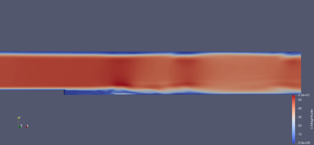 Here, we see the velocity distribution and the turbulent effects in the wake of the step.
Velocity Distribution at different x locations near the step: 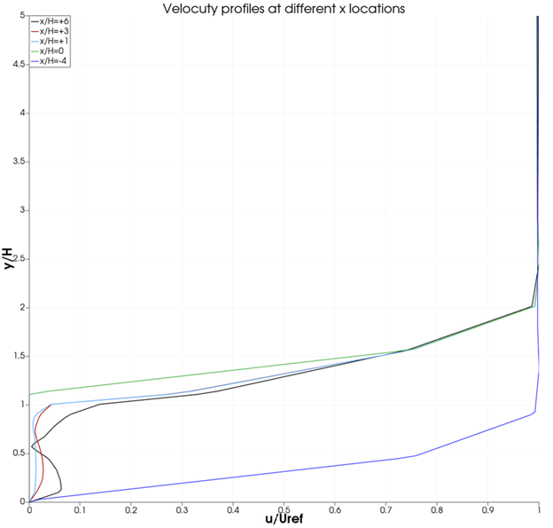
The velocity profile before the step shows a gradual increase from the walls to the center channel. Since the flow has no irregularities, the trend above is smooth and can also be corroborated with the velocity profile in the model above. The profile at the step shows the same trend as the profile before the step, as there are no irregularities in the flow except the distance between the locations. The after the step show irregularities in flow which indicates the turbulence and gradually increase and settle asymptomatically at the center channel.
Pressure coefficient over the lower wall: 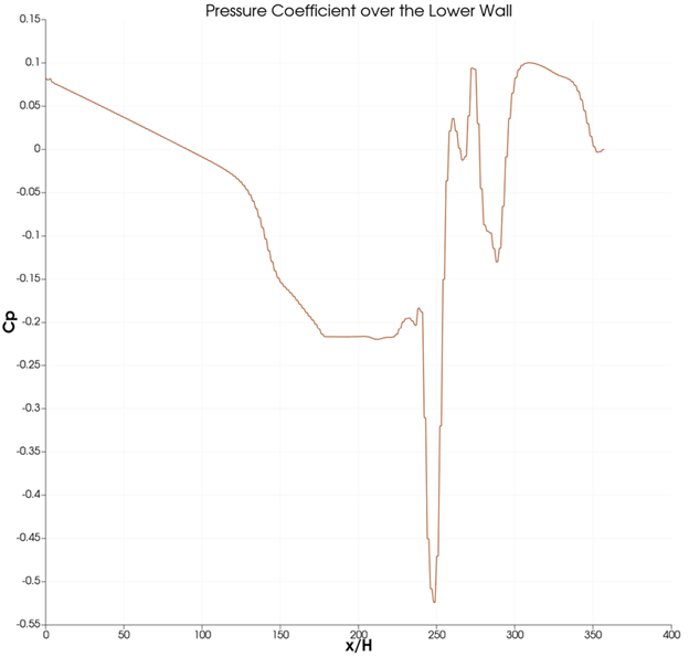
The above plot consists of the pressure coefficient which is captured along the lower wall of the backward step model. The trend starts with a high pressure coefficient value at the inlet and slowly decreases. It immediately falls at 200 x/H length and this is where the step is located. The following trend from the step corroborates the effects of turbulence and finally reaches an asymptotic value of 0.
Friction coefficient over the lower wall: 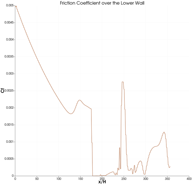
The above plot consists of the friction coefficient which is captured along the lower wall of the backward step model. The trend starts with a high value at the inlet and slowly decreases and falls drastically similar to the pressure plot, establishing the presence of the step. The following erratic trend from the step corroborates the effects of turbulence.
k-Epsilon Model:
Velocity distribution in the backward facing step: 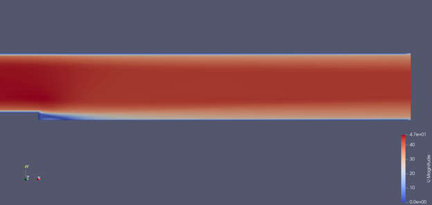
Velocity Distribution at different x locations near the step: 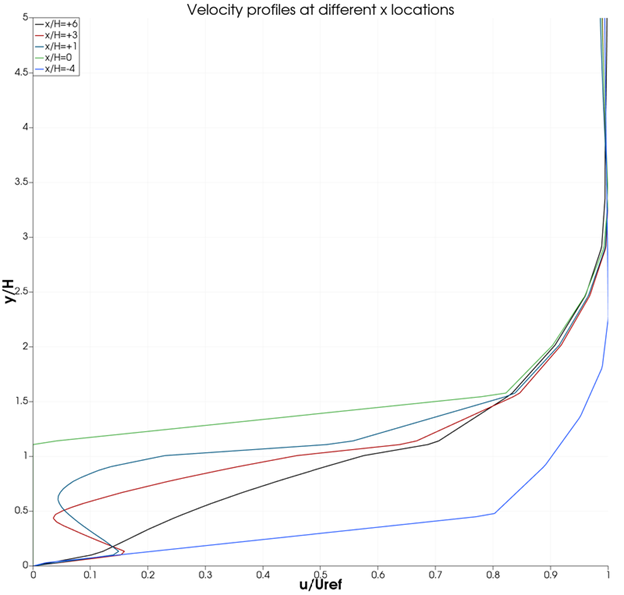
Similar to the velocity profiles of the Spalart Allmaras model, the profiles before and the step are the same. The profiles at +1 and +3 show significant changes when compared to the one at +6. From this we can interpret that the turbulence is prevalent at +1 and +3 profiles and at +6 the effects of turbulence is decreasing. It is also important to note that since this model is utilized for mean flow effects, it has successfully shown the results.
Pressure Distribution at different x locations near the step: 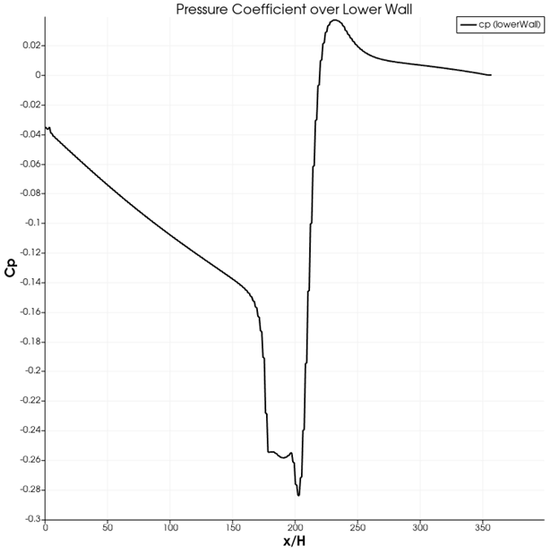
The above plot clearly depicts the effect of the step to the pressure coefficient and its substantial rise after it towards the end of the lower wall.
Friction coefficient over the lower wall:
Similarly to the pressure plot, the friction coefficient trend clearly depicts the presence and the effect of the backward step.
k-Omega Model
Velocity distribution in the backward facing step: 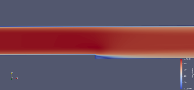
Velocity Distribution at different x locations near the step: 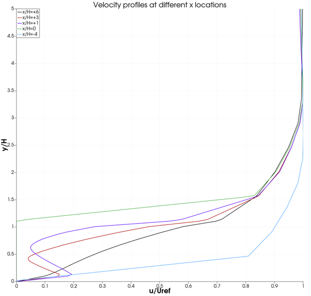
Similar to the velocity profiles of the above models, the profiles before and the step are the same. The profiles at +1 and +3 show significant changes when compared to the one at +6. From this we can interpret that the turbulence is prevalent at +1 and +3 profiles and at +6 the effects of turbulence is decreasing.
Pressure Distribution at different x locations near the step: 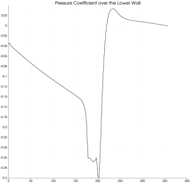
The above plot clearly depicts the effect of the step to the pressure coefficient and its substantial rise after it towards the end of the lower wall.
Friction coefficient over the lower wall: 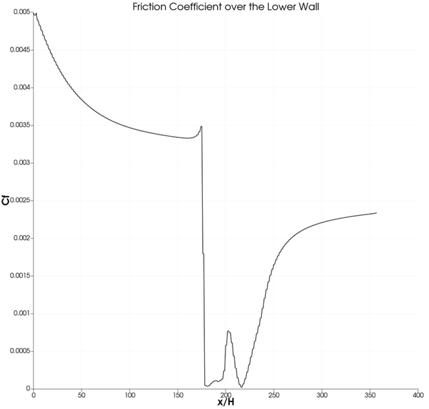
Similarly to the pressure plot, the friction coefficient trend clearly depicts the presence and the effect of the backward step.
Realizable k-Epsilon Model
Velocity distribution in the backward facing step: 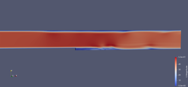
Velocity Distribution at different x locations near the step: 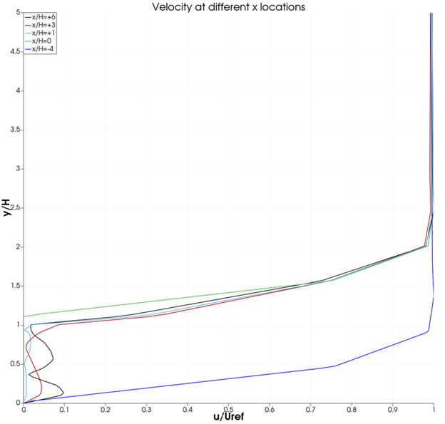
Following the same trend as the above models, the profiles before and the step are the same. The profiles at +1 and +3 show significant changes when compared to the one at +6. From this we can interpret that the turbulence is prevalent at +1 and +3 profiles and at +6 the effects of turbulence is decreasing.We also see that the effect of turbulence is more erratic here when compared to the other models. It is also important to note that since this model is utilized for planar flow effects, it has successfully shown the results.
Pressure Distribution at different x locations near the step: 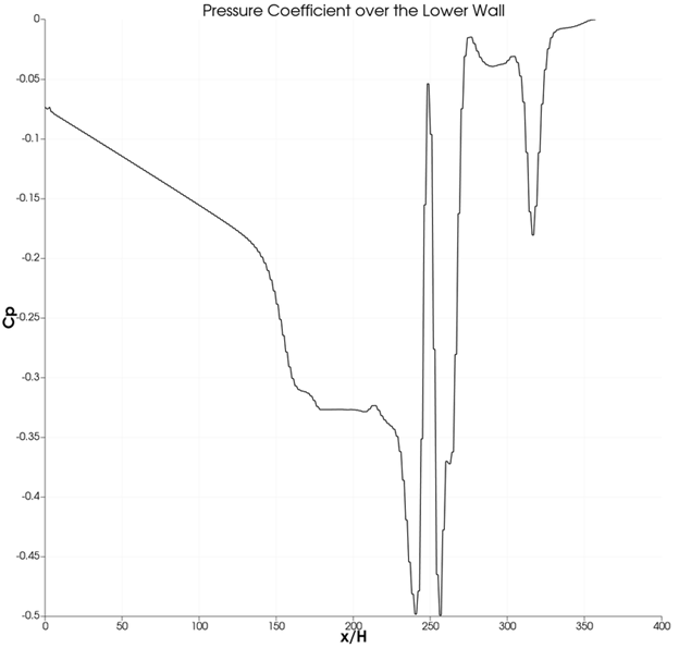
In the above plot, we can see that the pressure is greatly affected after the step and undergoes big changes.
Friction coefficient over the lower wall: 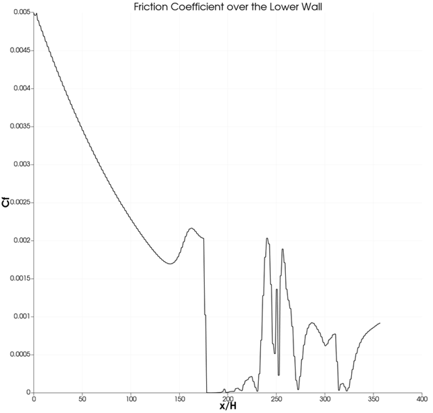
In the above plot, we can see that the friciton coefficient is very erratic and oscillating after the step and further down the lower wall.
Discussion and Inference:-
As we go further into the discussion there is an important thing to understand here. Implementing different turbulence models for a specific case can only bring results similar to what the model was designed for. Hence, the data visalisation we observe above are the interpretations of the models themselves.
The velocity comparison plots follow almost similar trends in all of the models except for the profiles \(x/H = +1, +3\). These profiles specifically show more accurate results for the Spalart- Allmaras and the realizable \(k-\epsilon\) models. This is because these models were developed to predict more accurate physics behind mean flows than the flows with low reynolds number regions i.e the flows near the wall region.
For the pressure and friction coeficient plots, among all of the above models, Spalart Allmaras and realizable \(k-\epsilon\) models show more adverse effects as they are supposed to. This should also be the case for the \(k-\omega\) model since it is made to predict flows near the wall or the boundary region. But the trend remains the same due to the inital conditions that do not effect the model to produce the said results.